


House prices and spam detection are common first machine learning projects. What else can you build?
Here are five Python projects to try, from recommending movies to extracting tables from PDFs. I ran all five on a CPU. Open the Colab notebook to run the code and see the results.
Let’s get into it.
1. Build a Recommendation System That Learns from User Behavior
Imagine someone browsing a movie application. Their older interactions are mostly comedy movies, but their recent activity involves science fiction.
What should the application recommend next?
A system that summarizes their overall preferences might continue suggesting comedy. A sequential recommendation system can use the order of interactions to represent their changing interests.
The project is to build a recommendation engine that accepts a user’s movie interaction history and suggests what they might explore next.
Train a small sequential recommender
We can start with MovieLens 100K, a small public benchmark containing movie ratings and timestamps. Here, an interaction means submitting a rating; it does not necessarily mean the person watched the movie at that time.
For the example below, we use PyTorch to train a small GRU (gated recurrent unit). It reads an ordered movie history and learns to predict the next interaction. RecBole is another option when you want to explore a wider collection of sequential models, including SASRec.
The following code downloads the dataset, builds histories of up to ten items, and trains on 6,000 history/next-item pairs. We reserve each user’s final two interactions when constructing the training examples. Five epochs keep this demonstration small.
python -m pip install torch pandas numpy matplotlib requestsimport io, zipfile, requests, random
import numpy as np
import pandas as pd
import matplotlib.pyplot as plt
import torch
from torch import nn
from torch.utils.data import TensorDataset, DataLoader
from IPython.display import display
random.seed(42); np.random.seed(42); torch.manual_seed(42)
torch.set_num_threads(2)
archive = zipfile.ZipFile(io.BytesIO(requests.get(
'https://files.grouplens.org/datasets/movielens/ml-100k.zip', timeout=60
).content))
events = pd.read_csv(archive.open('ml-100k/u.data'), sep='\t',
names=['user_id','item_id','rating','timestamp'])
movies = pd.read_csv(archive.open('ml-100k/u.item'), sep='|',
encoding='latin-1', header=None, usecols=[0,1], names=['item_id','title'])
sequences = events.sort_values(['user_id','timestamp','item_id']).groupby('user_id')['item_id'].agg(list)
n_items = int(events.item_id.max()) + 1
length = 10
def pad(history):
values = history[-length:]
return values + [0] * (length-len(values))
inputs, targets = [], []
for sequence in sequences:
training = sequence[:-2]
for end in range(1,len(training)):
inputs.append(pad(training[:end])); targets.append(training[end])
chosen = np.random.default_rng(42).choice(len(inputs), min(6000,len(inputs)), replace=False)
x = torch.tensor(np.array(inputs)[chosen], dtype=torch.long)
y = torch.tensor(np.array(targets)[chosen], dtype=torch.long)
class NextMovie(nn.Module):
def __init__(self):
super().__init__()
self.embedding = nn.Embedding(n_items,32,padding_idx=0)
self.gru = nn.GRU(32,32,batch_first=True)
self.output = nn.Linear(32,n_items)
def forward(self, history):
states,_ = self.gru(self.embedding(history))
last = history.ne(0).sum(1)-1
return self.output(states[torch.arange(len(history)),last])
model = NextMovie()
optimizer = torch.optim.Adam(model.parameters(),lr=0.003)
loader = DataLoader(TensorDataset(x,y),batch_size=128,shuffle=True)
losses=[]
for epoch in range(5):
total=0
for batch,label in loader:
optimizer.zero_grad()
loss=nn.functional.cross_entropy(model(batch),label)
loss.backward(); optimizer.step()
total+=loss.item()*len(batch)
losses.append(total/len(x))
user_id=sequences.index[0]; history=sequences.loc[user_id][:-2]
model.eval()
with torch.inference_mode():
scores=model(torch.tensor([pad(history)]))[0]
scores[0]=-torch.inf; scores[list(set(history))]=-torch.inf
ids=scores.topk(5).indices.tolist()
lookup=movies.set_index('item_id').title
recommendations=pd.DataFrame({'Rank':range(1,6),'Movie':[lookup.loc[i] for i in ids]})
print('PROJECT 1 | Sequential movie recommendations')
print(f'Trained a small GRU on {len(x):,} history/next-item pairs; CPU; 5 epochs.')
print('Recent rating interactions: '+ ' → '.join(lookup.loc[i] for i in history[-3:]))
display(recommendations)
fig,ax=plt.subplots(figsize=(10,3.5))
ax.barh(recommendations.Movie[::-1],range(1,6),color='#2c7fb8')
ax.set_title('Next movies suggested from an ordered rating history')
ax.set_xlabel('Display rank (5 = first recommendation)')
plt.tight_layout(); plt.savefig('01-sequential-result.png',dpi=160); plt.show()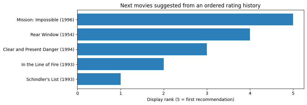
In this run, the first recommendation was Mission: Impossible (1996), followed by Rear Window (1954). The model excludes padding and previously rated movies when creating the list.
Let’s see what happens if we reverse the last ten ratings. Run this after the first example to compare both orders with the same trained model.
recent = history[-length:]
with torch.inference_mode():
    ranked = model(torch.tensor([pad(recent), pad(recent[::-1])]))
    ranked[:, 0] = -torch.inf
    ranked[:, list(set(history))] = -torch.inf
    normal, reversed_order = ranked.topk(5, dim=1).indices.tolist()

comparison = pd.DataFrame({
    'Rank': range(1, 6),
    'Original order': [lookup.loc[i] for i in normal],
    'Reversed order': [lookup.loc[i] for i in reversed_order],
})
print(comparison.to_string(index=False))
print('Titles in both top fives:', len(set(normal) & set(reversed_order)))
Here are the two rankings from the run.
Rank  Original order                    Reversed order
1     Mission: Impossible (1996)        Conspiracy Theory (1997)
2     Rear Window (1954)                People vs. Larry Flynt, The (1996)
3     Clear and Present Danger (1994)   Devil’s Advocate, The (1997)
4     In the Line of Fire (1993)        Mission: Impossible (1996)
5     Schindler’s List (1993)           Broken Arrow (1996)

Titles in both top fives: 1
Conspiracy Theory came first in the reversed list. Mission: Impossible dropped to fourth and was the only movie in both top fives. The model received the same ten ratings in both cases, so the order alone changed most of the recommendations for this user.
2. Build a Machine Learning System That Learns from New Data
Many tutorials collect a dataset, train a model, and stop learning once prediction begins. Transaction systems are different: observations keep arriving.
For this project, we would simulate transactions arriving one at a time. The model predicts processing time and updates after the actual time becomes available.
This introduces online or incremental learning. Instead of refitting the entire collected dataset, we update the model with individual observations.
Create a local transaction stream
River provides Python tools for incremental learning. Its estimators commonly expose predict_one() for prediction and learn_one() for updating. The linear regression documentation also demonstrates combining the estimator with an incremental scaler.
First, install the packages in your project environment:
python -m pip install river pandas matplotlib
Next, create fictional transactions with a fixed random seed:
import random
import pandas as pd
from river import linear_model, preprocessing

rng = random.Random(42)
model = (
    preprocessing.StandardScaler()
    | linear_model.LinearRegression()
)
history = []

for transaction_id in range(1000):
    x = {
        "amount": rng.uniform(5, 200),
        "items": rng.randint(1, 10),
    }
    prediction = model.predict_one(x)

    item_effect = 0.4 if transaction_id < 500 else 0.8
    actual_time = (
        2 + 0.02 * x["amount"]
        + item_effect * x["items"]
        + rng.gauss(0, 0.2)
    )

    history.append({
        "transaction_id": transaction_id,
        "prediction": prediction,
        "actual_time": actual_time,
    })
    model.learn_one(x, actual_time)

results = pd.DataFrame(history)
results.to_csv("stream_results.csv", index=False)
print(results.tail())
The order inside the loop matters. We make the prediction before revealing the outcome, then let the model learn from that observation.
Halfway through the simulation, the effect of item count changes. This represents a fictional operational change, such as an additional processing step for every item.
Inspect how the model changes
Run the following after the previous example:
import matplotlib.pyplot as plt

results.set_index("transaction_id")[[
    "prediction", "actual_time"
]].rolling(30).mean().plot(figsize=(10, 4))
plt.axvline(500, color="black", linestyle="--")
plt.ylabel("Processing time")
plt.tight_layout()
plt.show()
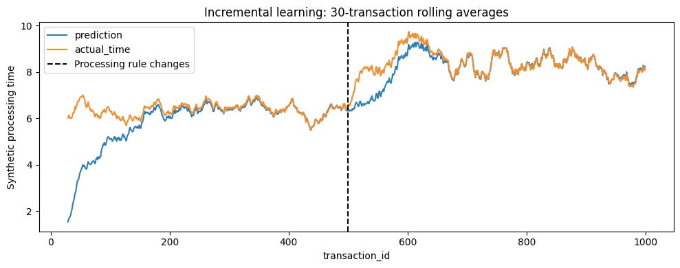
At transaction 500, the simulated time per item doubles from 0.4 to 0.8. In the plot, the actual processing time rises first. The predictions lag for a while, then move closer to the actual times as the model learns from transactions under the new rule.
3. Build a Multimodal Search Engine for Images and Text
Suppose we have a folder of flower photographs and want to find images matching “a yellow flower with long petals.”
Filename search would require useful descriptions to exist already. Image-text embeddings let us search the visual content instead.
An embedding is a numerical representation of an input. Models trained on image-text pairs learn image and language representations that can be compared in a shared space.
Our application would encode the image collection once, encode the user’s sentence, and rank images by similarity.
Prepare a small image collection
We can use OpenCLIP with the ViT-B-32 architecture and laion2b_s34b_b79k pretrained weights.
For images, download and extract the TensorFlow Flowers archive. The dataset catalog describes its 3,670 images and approximately 218 MiB download. TensorFlow itself is unnecessary here.
Keep flower_photos beside the script and retain the archive’s LICENSE.txt and image attribution records when sharing photographs.
Install the packages:
python -m pip install open_clip_torch torch pillow numpy matplotlib
The following example samples images from each category:
from pathlib import Path
import matplotlib.pyplot as plt
import numpy as np
import open_clip
import torch
from PIL import Image

model, _, preprocess = open_clip.create_model_and_transforms(
    "ViT-B-32", pretrained="laion2b_s34b_b79k"
)
tokenizer = open_clip.get_tokenizer("ViT-B-32")
model.eval()

paths = []
for folder in sorted(Path("flower_photos").iterdir()):
    if folder.is_dir():
        paths.extend(sorted(folder.glob("*.jpg"))[:20])
if not paths:
    raise ValueError("No images found in flower_photos.")

vectors = []
with torch.inference_mode():
    for path in paths:
        with Image.open(path) as image:
            batch = preprocess(image.convert("RGB")).unsqueeze(0)
        vector = model.encode_image(batch)
        vector /= vector.norm(dim=-1, keepdim=True)
        vectors.append(vector.cpu().numpy()[0])

    query = tokenizer(["a yellow flower with long petals"])
    query_vector = model.encode_text(query)
    query_vector /= query_vector.norm(dim=-1, keepdim=True)

scores = np.stack(vectors) @ query_vector.cpu().numpy()[0]
best = np.argsort(scores)[::-1][:5]

fig, axes = plt.subplots(1, len(best), figsize=(15, 3))
for ax, index in zip(np.atleast_1d(axes), best):
    with Image.open(paths[index]) as image:
        ax.imshow(image.convert("RGB"))
    ax.axis("off")
plt.tight_layout()
plt.show()
We normalize each embedding so the dot product gives cosine similarity. The code then displays the five highest-ranked photographs.
A CPU can process the small collection, although initial encoding may be slow. The first run downloads several hundred megabytes of weights, and PyTorch requires additional disk space.
OpenCLIP’s software is MIT licensed. Separately, the selected model card labels its weights MIT and describes research-use guidance and deployment limitations. Image permissions are a third, separate consideration.
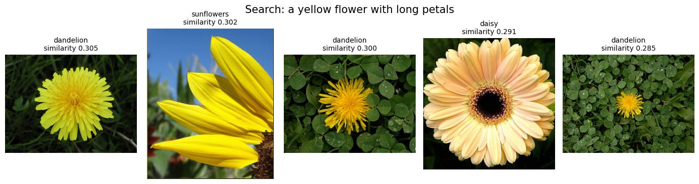
The dandelion came first at 0.305, just ahead of the sunflower at 0.302. Both match the color, and the sunflower is a closer match for the long petals. For a search like this, I would show several results so the user can pick the image that fits what they had in mind.
4. Build a Knowledge Graph That Predicts Missing Relationships
Imagine a dataset containing companies, components, and suppliers. We know some relationships, but others are missing.
Could a model suggest which connections are worth exploring?
A knowledge graph stores entities and relations as triples: a head entity, a relation, and a tail entity. For example, Supplier_A → supplies → Component_B is one triple.
Knowledge graph embedding models represent these entities and relationships numerically. Training encourages observed relationships to receive suitable scores, allowing the model to rank possible missing connections.
Train a small graph model
PyKEEN provides knowledge graph embedding tools and small benchmark datasets. We would use Nations, a historical dataset of countries and relationships.
Use a supported Python environment; the current repository specifies Python 3.11 or newer. Then install the package:
python -m pip install pykeen
Let’s train TransE and request possible tail entities for a relationship:
from pykeen.datasets import Nations
from pykeen.pipeline import pipeline
from pykeen.predict import predict_target

dataset = Nations()
result = pipeline(
    dataset=dataset,
    model="TransE",
    model_kwargs={"embedding_dim": 32},
    training_kwargs={"num_epochs": 30},
    random_seed=42,
    device="cpu",
)

predictions = predict_target(
    model=result.model,
    head="uk",
    relation="conferences",
    triples_factory=dataset.training,
)
unseen = predictions.filter_triples(dataset.training)
print(unseen.df.head(5))
This follows the documented target-prediction workflow.
TransE learns a representation where a relation moves us from the head entity toward the tail entity. The query above leaves the tail unspecified so the model can rank candidates.
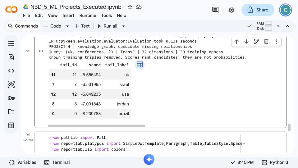
The UK came first in its own results. If we only want ties between different countries, keep rows where tail_label != "uk". Israel then moves to the top of the displayed list, followed by the US. These are the first two candidates I would check against the conference records.
5. Build an AI-Powered Document Intelligence System
Many business datasets arrive inside PDF reports. Before analyzing them with pandas, we need to recover the text, tables, and their organization.
This project turns a local report into readable document content and separate analytical tables.
Document intelligence involves identifying structure such as headings, table regions, and reading order. That structure helps preserve meaning when we move information into Python.
Convert a fictional business report
Docling supports local document conversion using specialized models for tasks such as layout analysis and table structure recognition.
For the first version, create a short report in a word processor and export it as report.pdf. Add a heading, a paragraph, and a table containing Product, Units, and Revenue. In the executed notebook, ReportLab generates this fictional report directly: Notebook (120 units, $1,800), Pen set (80 units, $640), and Desk organizer (35 units, $875). The notebook includes the generation code, so no private report is required.
Install the packages:
python -m pip install docling pandasThen convert the report:
from pathlib import Path
from docling.document_converter import DocumentConverter

output = Path("document_output")
output.mkdir(exist_ok=True)

converter = DocumentConverter()
result = converter.convert(Path("report.pdf"))
document = result.document

(output / "report.md").write_text(
    document.export_to_markdown(), encoding="utf-8"
)

for index, table in enumerate(document.tables, start=1):
    frame = table.export_to_dataframe(doc=document)
    frame.to_csv(output / f"table_{index}.csv", index=False)
    print(f"Table {index}")
    print(frame.head())
The code follows Docling’s official table-export example. We save the document as Markdown and each detected table as a CSV file.
Docling’s software is MIT licensed. Its model repository separately lists CDLA-Permissive-2.0 and Apache-2.0 licenses. Optional models and OCR components can have their own terms.
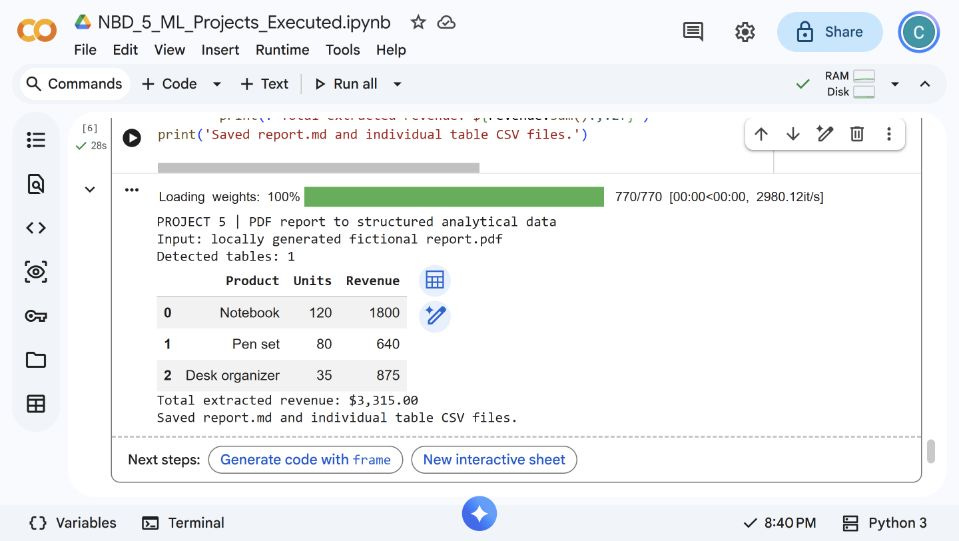
With table_1.csv in pandas, we can add up the three rows and get 235 units sold and $3,315 in revenue.
Conclusion
Machine Learning offers many projects beyond the familiar classification and regression tutorials. In this article, we have used Python to build five examples.
Recommend movies from an ordered rating history.
Update a model as new transactions arrive.
Search for photos using a text description.
Rank possible connections in a knowledge graph.
Extract tables from a PDF for analysis in pandas.
Choose the project that interests you most and start with the small version in Colab. Once you have a working result, you can adapt it to your own data.
I hope it helps!
Continue Learning with Non-Brand Data
If you want more practical examples in Data Science, Machine Learning, and AI, you can subscribe to Non-Brand Data.
The paid subscription includes more detailed tutorials, written courses, notebooks, and code.
If you want to discuss a Data Science project, a technical challenge, or what to focus on next in your career, I also offer 1-on-1 mentorship through MentorCruise.