5 Must-Know Dimensionality Reduction Techniques via Prince

Reducing features is good for your data science project

Reducing features is good for your data science project

Photo by Alexander Schimmeck on Unsplash

According to Wikipedia, Dimensionality Reduction is a transformation of High-Dimensionality space data into a Low-dimensionality space.

In other words, Dimensionality Reduction transforms data from a high number of features into a lower number of features. Let’s say from one hundred features into two features.

But why do we need Dimensionality Reduction? Isn’t it okay if we have many features for our Machine Learning model? Well, technically yes, but only until a certain point. More features might increase your metric, but it will peak somewhere and going down after that.

Furthermore, there are a few problems when we have too many features, including:

• A higher number of features increase variance in data, which could cause overfitting — Especially where the number of observations is less than the amount of the features present.

• The density and distance between data become less meaningful, which means the distance between data is equidistant or equally similar/different. This affecting the clustering and outlier detection as critical information from the data is undervalued.

• Combinatorial Explosion or a large number of values would lead to a computationally intractable problem where the process just takes too long to finish.

And some other problems, but you get the point. Too many features are not useful. That is why we need the Dimensionality Reduction technique.

You could think that the Dimensionality Reduction technique results as an intermediate step before the modeling part; Either your aim to clustering or prediction. Whether you only want to see the hidden underlying variation or use the result as another feature is your discretion.

Speaking of the result, all the result of these Dimensionality Reduction techniques is Singular Value Decomposition or SVD. This term would be found loosely in the article. I would not dwell too much here as SVD only dealt with the matric decomposition as a process rather than the main focus.

Minds that knowledge and business understanding never beat any kind of technique. It is better to have many relevant features rather than transform the not-so-relevant features although the point of Dimensional Reduction is to find that relevance in the feature space.

There are few Python Package out there dealing with the Dimensionality Reduction; one example is the prince package. In this article, I would outline the five Dimensionality Reduction techniques available in the prince package.

Dimensionality Reduction Techniques

The prince package branded itself as a Python factor analysis library. While not all Dimensionality Techniques is a factor analysis method, some are related. That is why the prince package, including the techniques that also associated with the factor analysis.

The techniques available for Dimensionality Reduction by the prince package are:

• Principal component analysis (PCA)

• Correspondence analysis (CA)

• Multiple correspondence analysis (MCA)

• Multiple factor analysis (MFA)

• Factor analysis of mixed data (FAMD)

In this article, I would not explain the theory of each technique in detail as I plan to create a more detailed article about it. Instead, I would give a short overview of the techniques and when you should apply it along with the example.

When to use the technique is depending on the features, below is the summarized table of when to apply the technique according to the prince package.

Table created by the author

Some note about the prince is that the prince package uses a randomized version of Singular Value Decomposition (SVD). Which is much faster than using the more commonly full approach, but the result might contain small inherent randomness. Most of the time, you did not need to worry about it, but if you want reproducible results then you should set the random_state parameter.

The randomized version of SVD is an iterative method and each of Prince’s algorithms applying SVD, they all possess a n_iter parameter that controls the number of iterations used for computing the SVD. In general, the algorithm converges very quickly, so using a low n_iter is recommended although a higher number could give a more precise result but with longer computation time.

Now, before we start, let’s install the package first.

pip install prince

1. Principal component analysis (PCA)

I think that PCA is the most introduce and the textbook model for the Dimensionality Reduction concept. PCA is a standard tool in modern data analysis because it is a simple non-parametric method for extracting relevant information from confusing data sets.

PCA aims to reduce complex information and provide a simplified structure hidden underneath the higher dimension. The primary benefit of PCA arises from calculating each dimension’s importance for describing data set variability. For example, six dimensions of data could have the majority of variation exist in one dimension. You could read the tutorial paper here if you want to inquire more about PCA and their limitation.

So, when would we use PCA to reduce the dimension? According to the prince guideline, it is when all the dimensions are numerical (all numerical features). Let’s try it with the dataset example.

#Importing the necessary package

import pandas as pdimport seaborn as snsfrom prince import PCA

#Dataset preparation with only numerical features

mpg = sns.load_dataset('mpg')

mpg.dropna(inplace=True)mpg_test = mpg.drop(['name', 'origin'], axis =1, inplace = True)mpg_test.head()

Now we have the mpg dataset with all numerical features. Let’s try to applying PCA into the dataset to reduce the features into two principal components. Note that you could set principal components as many as the number of features you feed into the model. In this case, it is seven, but it means no Dimensionality reduction at all.

#Setup our PCA, n_components control the number of the dimensionpca =PCA(n_components = 2, n_iter = 3, random_state = 101)

Training and transform our datapca.fit(mpg_test)mpg_pca = pca.transform(mpg_test)mpg_pca.head()

With this, we have reduced our seven dimension dataset into two-dimension (two PC), but how much variation this two-dimension explained the original dimension?

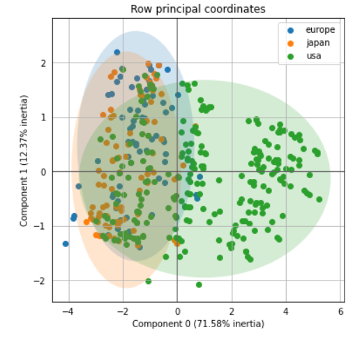
pca.explained_inertia_

It seems PC1 explained around 71%, and PC2 explained about 12%, so our two-dimension feature explained about 83% of the original dimension. That is not too bad. We could try to visualize our two PC as well with additional labels. Let’s try it with the ‘origin’ feature as the label.

ax = pca.plot_row_coordinates(mpg_test,      color_labels=mpg['origin'])

The two-dimension features could help separate the USA class and the other, although Europe and Japan label is a little bit harder.

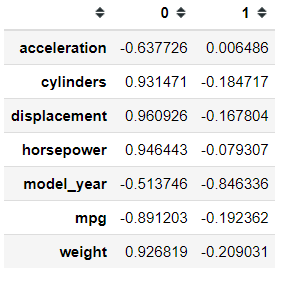
Let’s try another method PCA from prince offers. We can obtain the correlations between the original variables and the principal components.

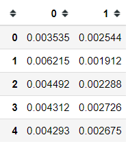
pca.column_correlations(mpg_test)

I am not sure which correlation method, but I am assuming it is the Pearson Correlation. We can also know how much each observation contributes to each principal component.

pca.row_contributions(mpg_test).head()

2.Correspondence Analysis (CA)

CA is a Dimensionality Reduction technique that traditionally applied to the contingency tables. It transforms data in a similar manner as PCA, where the central result is SVD. The inherent properties of CA who need the data to be in contingency tables mean it more appropriate to apply CA to categorical features. Let’s try it with a dataset example.

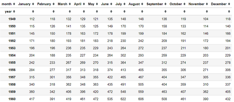
#Creating Contigency tables

flights = sns.load_dataset('flights')pivot = flight.pivot_table(values = 'passengers', index ='year' ,columns =  'month' )

This is our flight data contingency table, as we can see there is so much information here. We would use CA to reduce the dimension and extract additional insight there.

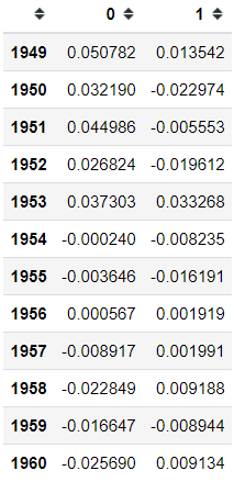
#Preparing CA

from prince import CAca = CA(n_components=2,n_iter=3,random_state=101 )

#Fitting the dataca.fit(pivot)

Unlike PCA, there is no data transformation, so we need to access the result from the class itself. Let’s try to get the row values (The row coordinate).

ca.row_coordinates(pivot)

Above is the variation information of the contingency table with the respect of the row (in this case, the year). If you want information from the column perspective, we could do it as well with the following code.

ca.column_coordinates(pivot)

And if you want to plot the coordinates, you could do it with the following code.

ax = ca.plot_coordinates(X = pivot, figsize = (6,6))

By plotting the coordinate, we could have a sense of where our data actually lies. We can see where the data tend to group together. This is how we get the hidden insight from the contingency table.

As an addition, you could access the variation explained by CA using the following code.

ca.explained_inertia_

3.Multiple correspondence analysis (MCA)

MCA is an extension of the CA for more than two categorical features (three or more). Which means MCA is applicable specific to categorical features. The idea of MCA is to applying CA into the one-hot encoded version of the dataset. Let’s try using a dataset example for now.

#Dataset preparation

tips = sns.load_dataset('tips')tips.drop(['total_bill', 'tip'], axis =1, inplace = True)

Above is the dataset contain only categorical features we would use (size feature is considered as categorical). Let’s try to apply MCA to the dataset.

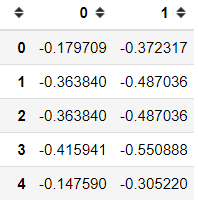
from prince import MCAmca = MCA(n_components = 2, n_iter = 3, random_state = 101)

mca.fit(tips)tips_mca = mca.transform(tips)tips_mca.head()

The result is like the PCA or CA result, two principal components with SVD result as the values. Just like previous techniques, we could plot the coordinates into a two-dimension graph.

mca.plot_coordinates(X = tips)

MCA has the same method with CA to acquire its column and row coordinates, and the plot above summarizes it all. We can see the colored one is the column coordinate and greyscale is the row coordinate. We can see that there seems a two kind of data clustering, the left side, and the right side.

Finally, you could access the variance explained by the model using the following code.

mca.explained_inertia_

4.Multiple factor analysis (MFA)

Multiple factor analysis (MFA) seeks the common structures present in all the features. MFA is used when you have a group of numerical or categorical features. This is because MFA is used to analyze a set of observations described by several group features. The main goal of MFA is to integrate different groups of features describing the same observations.

For the dataset example, I would use the tutorial from the prince package. In the tutorial dataset, it is about three experts give their opinion on six different wines. Opinion for each wine is recorded as a feature, and we want to consider the separate opinions of each expert while also having a global overview of each wine. MFA is suitable for this analysis.

Let’s try to set up the data.

X = pd.DataFrame(data=[         [1, 6, 7, 2, 5, 7, 6, 3, 6, 7],         [5, 3, 2, 4, 4, 4, 2, 4, 4, 3],         [6, 1, 1, 5, 2, 1, 1, 7, 1, 1],         [7, 1, 2, 7, 2, 1, 2, 2, 2, 2],         [2, 5, 4, 3, 5, 6, 5, 2, 6, 6],            [3, 4, 4, 3, 5, 4, 5, 1, 7, 5]     ],     columns=['E1 fruity', 'E1 woody', 'E1 coffee',              'E2 red fruit', 'E2 roasted', 'E2 vanillin', 'E2 woody',              'E3 fruity', 'E3 butter', 'E3 woody'],     index=['Wine {}'.format(i+1) for i in range(6)])X['Oak type'] = [1, 2, 2, 2, 1, 1]

Above is our dataset, opinion of each wine as the observation with Oak Type as an additional categorical variable. Now, using MFA in the prince, we need to specify the group category. So, let’s create one.

groups = {  'Expert #{}'.format(no+1): [c for c in X.columns if c.startswith('E{}'.format(no+1))] for no in range(3)}groups

With the group present, let’s try to applying MFA to reduce the dimension.

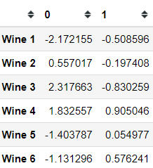
from prince import MFAmfa = MFA(groups = groups, n_components = 2, n_iter = 3, random_state = 101)

mfa.fit(X)mfa.transform(X)

Here we acquire the global row coordinates for each wine, where we already reduce the features into two-dimensions. Just like before, we could try to plot the row coordinates.

mfa.plot_row_coordinates(X=X, labels = X.index, color_labels=['Oak type {}'.format(t) for t in X['Oak type']])

We could see a clear separation of the wine and the closeness of each wine with the oak type as the label. If you want, we could also get the row coordinates of each data in the groups.

mfa.partial_row_coordinates(X)

And we could plot these groups row coordinates as well.

mfa.plot_partial_row_coordinates(X =X , color_labels=['Oak type {}'.format(t) for t in X['Oak type']])

When you need to access the model explained variance, you could access it just like previous techniques.

mfa.explained_inertia_

5.Factor Analysis of Mixed Data (FAMD)

Lastly, FAMD is a technique dedicated to the Dimensionality Reduction of data set containing both quantitative and qualitative features. It means FAMD is applied to data with both categorical and numerical features. It is possible by analyzing the similarity between observations by taking into account mixed types of features. Additionally, we can explore the association between all features.

Roughly speaking, the FAMD algorithm can be seen as a mix between PCA and MCA.

Let’s try it with a dataset example.

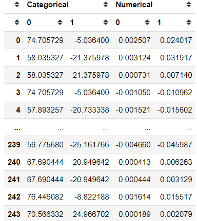
#Using the tips dataset, change the size feature to string objecttips = sns.load_dataset('tips')tips['size'] = tips['size'].astype('object')

from prince import FAMDfamd = FAMD(n_components =2, n_iter = 3, random_state = 101)

#I leave out tips as I want the sex feature as the labelfamd.fit(tips.drop('sex', axis =1))famd.transform(tips)

Just like before, we get the global row coordinates by reducing the dimension into two-dimensions. We could plot the row coordinates as well.

ax = famd.plot_row_coordinates(tips,color_labels=['Sex {}'.format(t) for t in tips['sex']] )

FAMD uses both PCA and MCA techniques in their analysis. That is why the building block of the coordinates is consisting of both the categorical and the numerical features. If you want to access these two analysis results, we could do it as well.

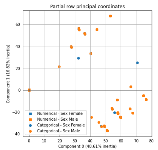
famd.partial_row_coordinates(tips)

And we could plot it as well.

ax = famd.plot_partial_row_coordinates(tips, color_labels=['Sex {}'.format(t) for t in tips['sex']])

Finally, if you want to know how much the variance explained by the model. You could access it as well with the following code.

famd.explained_inertia_

Conclusion

In this article, I have explained five different Dimensionality Reduction techniques provided by the prince package. It includes:

1. PCA (Principal Component Analysis)

2. CA (Correspondence Analysis)

3. MCA (Multiple Correspondence Analysis)

4. MFA (Multiple Factor Analysis)

5. FAMD (Factor Analysis of Mixed Data)

When to use the techniques is depends on the features you have.

I hope it helps!