5 SMOTE Techniques for Oversampling your Imbalance Data

Know your SMOTE ways to oversampled your data

Sep 14, 2020

Imbalance data is a case where the classification dataset class has a skewed proportion. For example, I would use the churn dataset from Kaggle for this article.

We can see there is a skew in the Yes class compared to the No class. If we calculate the proportion, the Yes class proportion is around 20.4% of the whole dataset. Although, how you classify the imbalance data? The table below might help you.

There are three cases of Imbalance — Mild, Moderate, and Extreme; depends on the minority class proportion to the whole dataset. In our example above, we only have a Mild case of imbalanced data.

Now, why we need to care about imbalance data when creating our machine learning model? Well, imbalance class creates a bias where the machine learning model tends to predict the majority class. You don’t want the prediction model to ignore the minority class, right?

That is why there are techniques to overcome the imbalance problem — Undersampling and Oversampling. What is the difference between these two techniques?

Undersampling would decrease the proportion of your majority class until the number is similar to the minority class. At the same time, Oversampling would resample the minority class proportion following the majority class proportion.

In this article, I would only write a specific technique for Oversampling called SMOTE and various variety of the SMOTE.

Just a little note, I am a Data Scientist who believes in leaving the proportion as it is because it is representing the data. It is better to try feature engineering before you jump into these techniques.

SMOTE

So, what is SMOTE? SMOTE or Synthetic Minority Oversampling Technique is an oversampling technique but SMOTE working differently than your typical oversampling.

In a classic oversampling technique, the minority data is duplicated from the minority data population. While it increases the number of data, it does not give any new information or variation to the machine learning model.

For a reason above, Nitesh Chawla, et al. (2002) introduce a new technique to create synthetic data for oversampling purposes in their SMOTE paper.

SMOTE works by utilizing a k-nearest neighbor algorithm to create synthetic data. SMOTE first start by choosing random data from the minority class, then k-nearest neighbors from the data are set. Synthetic data would then made between the random data and the randomly selected k-nearest neighbor. Let me show you the example below.

The procedure is repeated enough times until the minority class has the same proportion as the majority class.

I omit a more in-depth explanation because the passage above already summarizes how SMOTE work. In this article, I want to focus on SMOTE and its variation, as well as when to use it without touching much in theory. If you want to know more, let me attach the link to the paper for each variation I mention here.

As preparation, I would use the imblearn package, which includes SMOTE and their variation in the package.

#Installing imblearn

pip install -U imbalanced-learn

1. SMOTE

We would start by using the SMOTE in their default form. We would use the same churn dataset above. Let’s prepare the data first as well to try the SMOTE.

If you realize from my explanation above, SMOTE is used to synthesize data where the features are continuous and a classification problem. For that reason, in this section, we only would try to use two continuous features with the classification target.

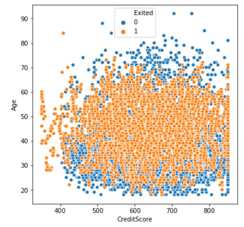
import pandas as pdimport seaborns as sns

#I read the csv churn data into variable called df. Here I would only use two continuous features CreditScore and Age with the target Exited

df_example = df[['CreditScore', 'Age', 'Exited']]sns.scatterplot(data = df, x ='CreditScore', y = 'Age', hue = 'Exited')

As we can see in the above scatter plot between the ‘CreditScore’ and ‘Age’ feature, there are mixed up between the 0 and 1 class.

Let’s try to oversampled the data using the SMOTE technique.

#Importing SMOTEfrom imblearn.over_sampling import SMOTE

#Oversampling the datasmote = SMOTE(random_state = 101)X, y = smote.fit_resample(df[['CreditScore', 'Age']], df['Exited'])

#Creating a new Oversampling Data Framedf_oversampler = pd.DataFrame(X, columns = ['CreditScore', 'Age'])df_oversampler['Exited']

sns.countplot(df_oversampler['Exited'])

As we can see in the graph above, class 0 and 1 now have a similar proportion. Let’s see how is it goes if we create a similar scatter plot like before.

sns.scatterplot(data = df_oversampler, x ='CreditScore', y = 'Age', hue = 'Exited')

Currently, we have the oversampled data to fill the area that previously was empty with the synthetic data.

The purpose of oversampling is, just as I stated before, to have a better prediction model. This technique was not created for any analysis purposes as every data created is synthetic, so that is a reminder.

For the reason above, we need to evaluate whether oversampling data leads to a better model or not. Let’s start by splitting the data to create the prediction model.

# Importing the splitter, classification model, and the metricfrom sklearn.linear_model import LogisticRegressionfrom sklearn.model_selection import train_test_splitfrom sklearn.metrics import classification_report

#Splitting the data with stratification

X_train, X_test, y_train, y_test = train_test_split(df_example[['CreditScore', 'Age']], df['Exited'], test_size = 0.2, stratify = df['Exited'], random_state = 101)

As an addition, you should only oversample your training data and not the whole data except if you would use the entire data as your training data. In case you want to split the data, you should split the data first before oversampled the training data.

#Create an oversampled training datasmote = SMOTE(random_state = 101)X_oversample, y_oversample = smote.fit_resample(X_train, y_train)

Now we have both the imbalanced data and oversampled data, let’s try to create the classification model using both of these data. First, let’s see the performance of the Logistic Regression model trained with the imbalanced data.

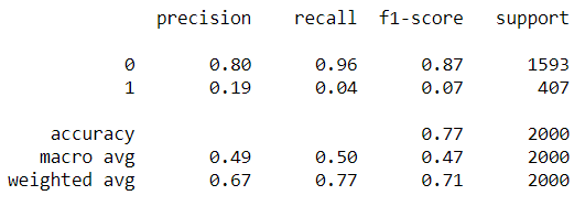
#Training with imbalance dataclassifier = LogisticRegression()classifier.fit(X_train, y_train)

print(classification_report(y_test, classifier.predict(X_test)))

As we can see from the metrics, our Logistic Regression model trained with the imbalanced data tends to predict class 0 rather than class 1. The bias is in our model.

Let’s see how is the result of the model trained with the oversampled data.

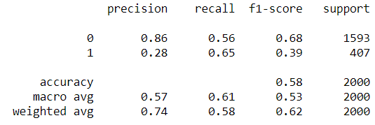
#Training with oversampled data

classifier_o = LogisticRegression()classifier_o.fit(X_oversample, y_oversample)

print(classification_report(y_test, classifier_o.predict(X_test)))

The model is doing better at predicted class 1 in this case. In this case, we could say that the oversampled data helps our Logistic Regression model to predict the class 1 better.

I could say that the oversampled data improve the Logistic Regression model for prediction purposes, although the context of ‘improve’ is once again back to the user.

2. SMOTE-NC

I have mention that SMOTE only works for continuous features. So, what to do if you have mixed (categorical and continuous) features? In this case, we have another variation of SMOTE called SMOTE-NC (Nominal and Continuous).

You might think, then, just transform the categorical data into numerical; therefore, we had a numerical feature for SMOTE to use. The problem is when we did that; we would have data that did not make any sense.

For example, in the churn data above, we had ‘IsActiveMember’ categorical feature with the data either 0 or 1. If we oversampled this data with SMOTE, we could end up with oversampled data such as 0.67 or 0.5, which does not make sense at all.

This is why we need to use SMOTE-NC when we have cases of mixed data. The premise is simple, we denote which features are categorical, and SMOTE would resample the categorical data instead of creating synthetic data.

Let’s try applying SMOTE-NC. In this case, I would select another feature as an example (one categorical, one continuous).

df_example = df[['CreditScore', 'IsActiveMember', 'Exited']]

In this case, ‘CreditScore’ is the continuous feature, and ‘IsActiveMember’ is the categorical feature. Then, let’s split the data just like before.

X_train, X_test, y_train, y_test = train_test_split(df_example[['CreditScore', 'IsActiveMember']],df['Exited'], test_size = 0.2,stratify = df['Exited'], random_state = 101)

Then, let’s create two different classification models once more; one trained with the imbalanced data and one with the oversampled data. First, let’s try SMOTE-NC to oversampled the data.

#Import the SMOTE-NCfrom imblearn.over_sampling import SMOTENC

#Create the oversampler. For SMOTE-NC we need to pinpoint the column position where is the categorical features are. In this case, 'IsActiveMember' is positioned in the second column we input [1] as the parameter. If you have more than one categorical columns, just input all the columns position

smotenc = SMOTENC([1],random_state = 101)X_oversample, y_oversample = smotenc.fit_resample(X_train, y_train)

With the data ready, let’s try to create the classifiers.

#Classifier with imbalance data

classifier = LogisticRegression()classifier.fit(X_train, y_train)

print(classification_report(y_test, classifier.predict(X_test)))

With the imbalance data, we can see the classifier favor the class 0 and ignore the class 1 completely. Then, how about if we trained it with the SMOTE-NC oversampled data.

#Classifier with SMOTE-NC

classifier_o = LogisticRegression()classifier_o.fit(X_oversample, y_oversample)

print(classification_report(y_test, classifier_o.predict(X_test)))

Just like with SMOTE, the classifier with SMOTE-NC oversampled data give a new perspective to the machine learning model to predict the imbalanced data. It wasn’t necessarily the best, but it was better than the imbalance data.

3. Borderline-SMOTE

Borderline-SMOTE is a variation of the SMOTE. Just like the name implies, it has something to do with the border.

So, unlike with the SMOTE, where the synthetic data are created randomly between the two data, Borderline-SMOTE only makes synthetic data along the decision boundary between the two classes.

Also, there are two kinds of Borderline-SMOTE; there are Borderline-SMOTE1 and Borderline-SMOTE2. The differences are simple; Borderline-SMOTE1 also oversampled the majority class where the majority data are causing misclassification in the decision boundary, while Borderline-SMOTE2 only oversampled the minority classes.

Let’s try the Borderline-SMOTE with our previous data. I would once more only using the numerical features.

df_example = df[['CreditScore', 'Age', 'Exited']]

The above picture is the difference between oversampling data with SMOTE and Borderline-SMOTE1. It might slightly look similar, but we could see there are differences where the synthetic data are created.

How about the performances for the machine learning model? Let us try it. First, as usual, we split the data.

X_train, X_test, y_train, y_test = train_test_split(df_example[['CreditScore', 'Age']], df['Exited'], test_size = 0.2,  stratify = df['Exited'], random_state = 101)

Then, we create the oversampled data by using Borderline-SMOTE.

#By default, the BorderlineSMOTE would use the Borderline-SMOTE1from imblearn.over_sampling import BorderlineSMOTE

bsmote = BorderlineSMOTE(random_state = 101, kind = 'borderline-1')

X_oversample_borderline, y_oversample_borderline = bsmote.fit_resample(X_train, y_train)

Lastly, let’s check the machine learning performance with the Borderline-SMOTE oversampled data.

classifier_border = LogisticRegression()classifier_border.fit(X_oversample_borderline, y_oversample_borderline)

print(classification_report(y_test, classifier_border.predict(X_test)))

The performance doesn’t differ much from the model trained with the SMOTE oversampled data. This means that we should focus on the features instead of oversampling the data.

Borderline-SMOTE is used the best when we know that the misclassification often happens near the boundary decision. Otherwise, we could stay use the usual SMOTE. If you want to read more about the Borderline-SMOTE, you could check the paper here.

4. Borderline-SMOTE SVM

Another variation of Borderline-SMOTE is Borderline-SMOTE SVM, or we could just call it SVM-SMOTE.

The main differences between SVM-SMOTE and the other SMOTE are that instead of using K-nearest neighbors to identify the misclassification in the Borderline-SMOTE, the technique would incorporate the SVM algorithm.

In the SVM-SMOTE, the borderline area is approximated by the support vectors after training SVMs classifier on the original training set. Synthetic data will be randomly created along the lines joining each minority class support vector with a number of its nearest neighbors.

What special about Borderline-SMOTE SVM compared to the Borderline-SMOTE is that more data are synthesized away from the region of class overlap. It focuses more on where the data is separated.

Just like before, let’s try to use the technique in the model creation. I would still use the same training data in the Borderline-SMOTE example.

from imblearn.over_sampling import SVMSMOTEsvmsmote = SVMSMOTE(random_state = 101)

X_oversample_svm, y_oversample_svm = svmsmote.fit_resample(X_train, y_train)

classifier_svm = LogisticRegression()classifier_svm.fit(X_oversample_svm, y_oversample_svm)

print(classification_report(y_test, classifier_svm.predict(X_test)))

The performance is once more not differ much, although I could say that the model in this time slightly favored the class 0 more than when we use the other technique but not too much.

It depends on you once again, what are your prediction models target are and the business affected by it. If you want to read more about the Borderline-SMOTE SVM, you could check the paper here.

5. Adaptive Synthetic Sampling (ADASYN)

ADASYN is another variation from SMOTE. ADASYN takes a more different approach compared to the Borderline-SMOTE. While Borderline-SMOTE tries to synthesize the data near the data decision boundary, ADASYN creates synthetic data according to the data density.

The synthetic data generation would inversely proportional to the density of the minority class. It means more synthetic data are created in regions of the feature space where the density of minority examples is low, and fewer or none where the density is high.

In simpler terms, in an area where the minority class is less dense, the synthetic data are created more. Otherwise, the synthetic data is not made so much.

Let’s see how the performance by using the ADASYN. I would still use the same training data in the Borderline-SMOTE example.

from imblearn.over_sampling import ADASYNadasyn = ADASYN(random_state = 101)

X_oversample_ada, y_oversample_ada = adasyn.fit_resample(X_train, y_train)

classifier_ada = LogisticRegression()classifier_ada.fit(X_oversample_ada, y_oversample_ada)

print(classification_report(y_test, classifier_ada.predict(X_test)))

As we can see from the model performance above, the performance is slightly worse than when we use the other SMOTE method.

The problems might lie in the outliers. Just like I stated before, ADASYN would focus on the density data where the density is low. Often time, the low-density data is an outlier. The ADASYN approach would then put too much attention on these areas of the feature space, which may result in worse model performance. It might be better to remove the outlier before using the ADASYN.

If you want to read more about ADASYN, you could check the paper here.

Conclusion

Imbalanced data is a problem when creating a predictive machine learning model. One way to alleviate this problem is by oversampling the minority data.

Instead of oversampling by replicating the data, we can oversample the data by creating synthetic data using the SMOTE technique. There are few variations of SMOTE, including:

SMOTE
SMOTE-NC
Borderline-SMOTE
SVM-SMOTE
ADASYN

I hope it helps!

Non-Brand Data

Discussion about this post