
Breaking down the agglomerative clustering process
Detailed step-by-step how to apply agglomerative clustering on your data

Detailed step-by-step how to apply agglomerative clustering on your data

If you did not recognize the picture above, it is expected as this picture mostly could only be found in the biology journal or textbook. What I have above is a species phylogeny tree, which is a historical biological tree shared by the species with a purpose to see how close they are with each other. In more general terms, if you are familiar with the Hierarchical Clustering it is basically what it is. To be precise, what I have above is the bottom-up or the Agglomerative clustering method to create a phylogeny tree called Neighbour-Joining.
Agglomerative Clustering
Introduction
In machine learning, unsupervised learning is a machine learning model that infers the data pattern without any guidance or label. Many models are included in the unsupervised learning family, but one of my favorite models is Agglomerative Clustering.
Agglomerative Clustering or bottom-up clustering essentially started from an individual cluster (each data point is considered as an individual cluster, also called leaf), then every cluster calculates their distance with each other. The two clusters with the shortest distance with each other would merge creating what we called node. Newly formed clusters once again calculating the member of their cluster distance with another cluster outside of their cluster. The process is repeated until all the data points assigned to one cluster called root. The result is a tree-based representation of the objects called dendrogram.
Just for reminder, although we are presented with the result of how the data should be clustered; Agglomerative Clustering does not present any exact number of how our data should be clustered. It is up to us to decide where is the cut-off point.

Let’s try to break down each step in a more detailed manner. For the sake of simplicity, I would only explain how the Agglomerative cluster works using the most common parameter.
Distance Measurements
We begin the agglomerative clustering process by measuring the distance between the data point. How it is calculated exactly? Let me give an example with dummy data.
#creating dummy dataimport pandas as pddummy = pd.DataFrame([[30,100,5], [18, 200, 2], [35, 150, 7], [48, 300, 4], [50, 200, 6]], index = ['Anne', 'Ben', 'Chad', 'Dave', 'Eric'], columns =['Age', 'Expense($)', 'Distance(KM)'])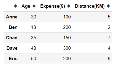
Let’s say we have 5 different people with 3 different continuous features and we want to see how we could cluster these people. First thing first, we need to decide our clustering distance measurement.
One of the most common distance measurements to be used is called Euclidean Distance.

Euclidean distance in a simpler term is a straight line from point x to point y. I would give an example by using the example of the distance between Anne and Ben from our dummy data.
In the dummy data, we have 3 features (or dimensions) representing 3 different continuous features. In this case, we could calculate the Euclidean distance between Anne and Ben using the formula below.

If we put all the numbers, it would be.

Using Euclidean Distance measurement, we acquire 100.76 for the Euclidean distance between Anne and Ben. Similarly, applying the measurement to all the data points should result in the following distance matrix.
import numpy as npfrom scipy.spatial import distance_matrix#distance_matrix from scipy.spatial would calculate the distance between data point based on euclidean distance, and I round it to 2 decimalpd.DataFrame(np.round(distance_matrix(dummy.values, dummy.values), 2), index = dummy.index, columns = dummy.index)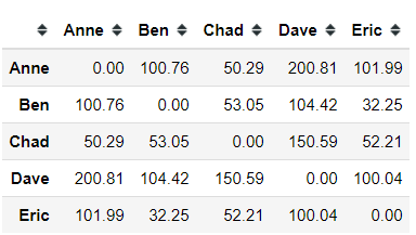
After that, we merge the smallest non-zero distance in the matrix to create our first node. In this case, it is Ben and Eric.
With a new node or cluster, we need to update our distance matrix.
Now we have a new cluster of Ben and Eric, but we still did not know the distance between (Ben, Eric) cluster to the other data point. How do we even calculate the new cluster distance? In order to do this, we need to set up the linkage criterion first.
Linkage Criterion
The linkage criterion is where exactly the distance is measured. It is a rule that we establish to define the distance between clusters.
There are many linkage criterion out there, but for this time I would only use the simplest linkage called Single Linkage. How it is work? I would show it in the picture below.
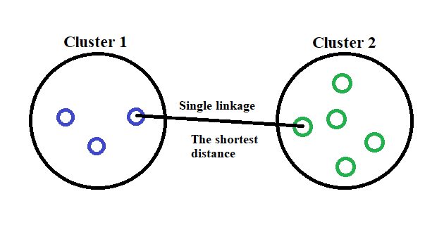
In a single linkage criterion we, define our distance as the minimum distance between clusters data point. If we put it in a mathematical formula, it would look like this.
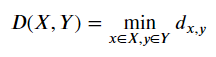
Where the distance between cluster X to cluster Y is defined by the minimum distance between x and y which is a member of X and Y cluster respectively.
Let us take an example. If we apply the single linkage criterion to our dummy data, say between Anne and cluster (Ben, Eric) it would be described as the picture below.
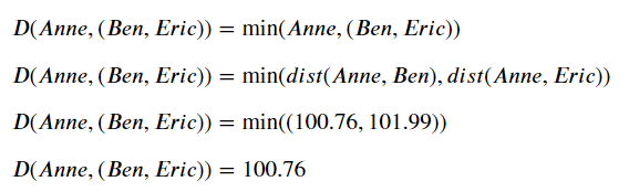
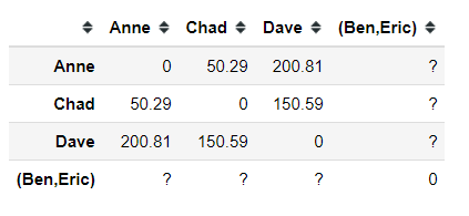
With a single linkage criterion, we acquire the euclidean distance between Anne to cluster (Ben, Eric) is 100.76. Applying the single linkage criterion to our dummy data would result in the following distance matrix.
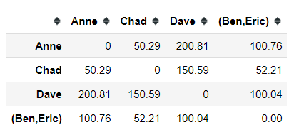
Now, we have the distance between our new cluster to the other data point. Although if you notice, the distance between Anne and Chad is now the smallest one. In this case, the next merger event would be between Anne and Chad.

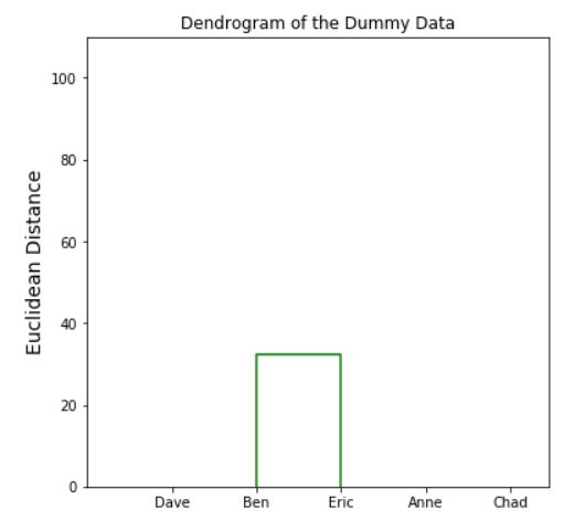
We keep the merging event happens until all the data is clustered into one cluster. In the end, we would obtain a dendrogram with all the data that have been merged into one cluster.
#importing linkage and denrogram from scipyfrom scipy.cluster.hierarchy import linkage, dendrogramimport matplotlib.pyplot as plt#creating dendrogram based on the dummy data with single linkage criterionden = dendrogram(linkage(dummy, method='single'), labels = dummy.index)plt.ylabel('Euclidean Distance', fontsize = 14)plt.title('Dendrogram of the Dummy Data')plt.show()
Determining the number of clusters
We already get our dendrogram, so what we do with it? We would use it to choose a number of the cluster for our data. Remember, dendrogram only show us the hierarchy of our data; it did not exactly give us the most optimal number of cluster.
The best way to determining the cluster number is by eye-balling our dendrogram and pick a certain value as our cut-off point (manual way). Usually, we choose the cut-off point that cut the tallest vertical line. I would show an example with pictures below.
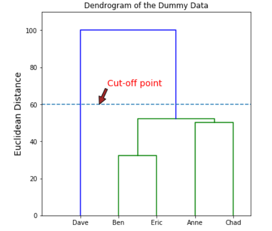
The number of intersections with the vertical line made by the horizontal line would yield the number of the cluster.
Choosing a cut-off point at 60 would give us 2 different clusters (Dave and (Ben, Eric, Anne, Chad)). Choosing a different cut-off point would give us a different number of the cluster as well. For example, if we shift the cut-off point to 52.
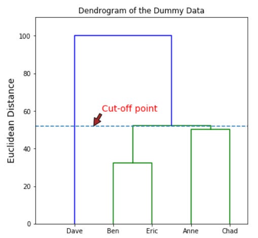
This time, with a cut-off at 52 we would end up with 3 different clusters (Dave, (Ben, Eric), and (Anne, Chad)).
In the end, we the one who decides which cluster number makes sense for our data. Possessing domain knowledge of the data would certainly help in this case.
And of course, we could automatically find the best number of the cluster via certain methods; but I believe that the best way to determine the cluster number is by observing the result that the clustering method produces.
Agglomerative clustering model
Let’s say I would choose the value 52 as my cut-off point. It means that I would end up with 3 clusters. With this knowledge, we could implement it into a machine learning model.
from sklearn.cluster import AgglomerativeClusteringaglo = AgglomerativeClustering(n_clusters=3, affinity='euclidean', linkage='single')aglo.fit_predict(dummy)The Agglomerative Clustering model would produce [0, 2, 0, 1, 2] as the clustering result. We could then return the clustering result to the dummy data. In my case, I named it as ‘Aglo-label’.
dummy['Aglo-label'] = aglo.fit_predict(dummy)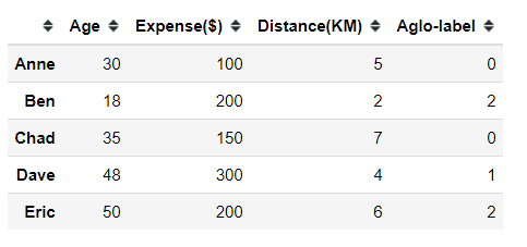
Now my data have been clustered, and ready for further analysis. It is necessary to analyze the result as unsupervised learning only infers the data pattern but what kind of pattern it produces needs much deeper analysis.
Conclusion
Agglomerative Clustering is a member of the Hierarchical Clustering family which work by merging every single cluster with the process that is repeated until all the data have become one cluster.
The step that Agglomerative Clustering take are:
Each data point is assigned as a single cluster
Determine the distance measurement and calculate the distance matrix
Determine the linkage criteria to merge the clusters
Update the distance matrix
Repeat the process until every data point become one cluster
With a dendrogram, then we choose our cut-off value to acquire the number of the cluster.
In the end, Agglomerative Clustering is an unsupervised learning method with a purpose to learn from our data. It is still up to us how to interpret the clustering result.
I provide the github link for the notebook here as further reference.