

Building a machine learning model for tabular data often starts with familiar methods such as Logistic Regression, Random Forest, or CatBoost. We train them on our data and compare their predictions to find a model that suits our problem.
TabPFN-3.5 gives us another option. It uses a pretrained model to make predictions from the examples we provide. I wanted to see how this approach compares with the models we already use, including how long we need to wait for the predictions.
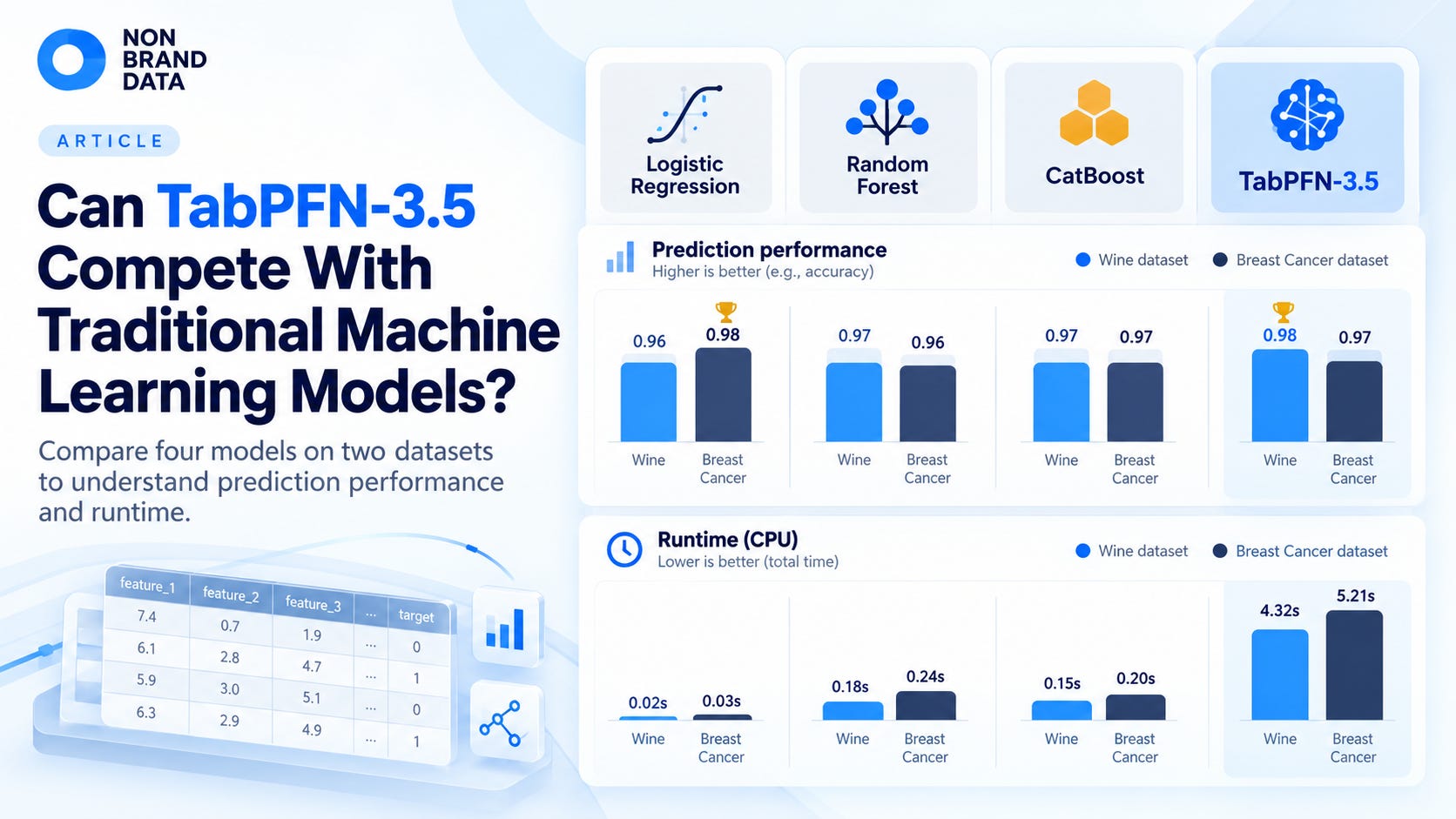
In this article, we will compare TabPFN-3.5 with Logistic Regression, Random Forest, and CatBoost on two datasets. We will look at their prediction performance and runtime, then discuss the limitations of the comparison.
Let’s get into it.
All the experiments are contained within this repository.
What makes TabPFN-3.5 different?
To understand this comparison, let’s first look at how TabPFN-3.5 uses our data. It takes labeled training examples as context and predicts the target for new rows. According to Prior Labs, the model was pretrained on synthetic tabular tasks, and the base checkpoint supports both classification and regression.
Prior Labs released TabPFN-3.5 on September 15, 2026. Its release report describes several variants, including Fast, Plus, and Thinking. For this comparison, I used the base model.
With that model, we still use the familiar fit() and predict_proba() methods in TabPFN. However, calling fit() does not train the foundation model from scratch. We provide context for a model that has already been pretrained, which differs from fitting Logistic Regression coefficients or building trees from our dataset.
This also affects how we compare runtime. We need to measure both fitting and prediction to see how long each model takes to produce results. Before we get to those measurements, let’s prepare the datasets and give every model the same train/test splits.
Preparing our comparison
We will use the Breast Cancer Wisconsin Diagnostic and Wine datasets included with scikit-learn. I chose them because we can load the data without a separate download. They also let us compare the models on a binary classification problem and a multiclass problem.

In Breast Cancer, we use measurements derived from digitized images of breast masses to predict malignant or benign labels. Wine gives us a different task: using chemical measurements to distinguish three cultivars. Both loaded datasets have numeric features and no missing values so that we can focus this comparison on complete numeric data.
Their small size makes the experiment easy to repeat, but it also limits what we can conclude about business datasets. We are using Breast Cancer as a classification exercise; these results don’t establish whether a model is suitable for clinical use.
With that scope in mind, let’s create our first train/test split:
from sklearn.datasets import load_breast_cancer
from sklearn.model_selection import train_test_split

data = load_breast_cancer(as_frame=True)
X_train, X_test, y_train, y_test = train_test_split(
 data.data,
 data.target,
 test_size=0.25,
 stratify=data.target,
 random_state=42
)
We keep 75% of the rows for training and 25% for testing. The stratify argument keeps the class proportions close to those in the full dataset.
In the notebook, we repeat this with seeds 42 through 46 for both datasets. Every model gets the same rows within each split. Four models across two datasets and five splits give us 40 evaluations.
Setting up the models
With our splits prepared, we can set up the models. For Logistic Regression, we put StandardScaler inside a pipeline:
from sklearn.pipeline import make_pipeline
from sklearn.preprocessing import StandardScaler
from sklearn.linear_model import LogisticRegression

model = make_pipeline(
 StandardScaler(),
 LogisticRegression(C=1.0, max_iter=2000, random_state=42)
)
model.fit(X_train, y_train)
probabilities = model.predict_proba(X_test)
The scaler learns from the training rows and applies that transformation to the test rows. We shouldn’t scale the full dataset before splitting because that would let test data influence preprocessing.
The other models receive the original numeric values. Alongside this pipeline, I used Random Forest, CatBoost, and TabPFN-3.5 with the following settings. I kept these configurations fixed without a hyperparameter search:

The results therefore describe these configurations, and tuning could change them. The settings also represent different amounts of work: four TabPFN ensemble members shouldn’t be treated as equivalent to four trees.
To make sure we test the intended TabPFN model, we select its version explicitly:
from tabpfn import TabPFNClassifier
from tabpfn.constants import ModelVersion

model = TabPFNClassifier.create_default_for_version(
 ModelVersion.V3_5,
 n_estimators=4,
 device=”cpu”,
 random_state=42,
 n_preprocessing_jobs=1,
 show_progress_bar=False
)
model.fit(X_train, y_train)
probabilities = model.predict_proba(X_test)
The Python package version is tabpfn==9.1.0, while the model we’re testing is TabPFN-3.5. Choosing ModelVersion.V3_5 keeps the experiment from depending on the package’s default model version.
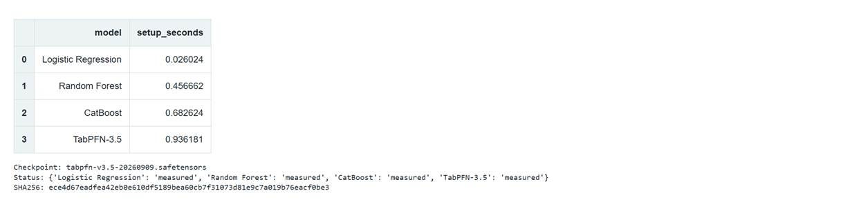
To make that choice reproducible, the notebook pins the TabPFN-3.5 checkpoint tabpfn-v3.5-20260909.safetensors and records its SHA256 hash. Before the first download, we need to accept the model license and enable authenticated access through Prior Labs. Keep the access key outside the notebook. Once the weights are available, inference runs locally. The setup output below confirms which checkpoint we used and that all four models ran.
Comparing prediction performance
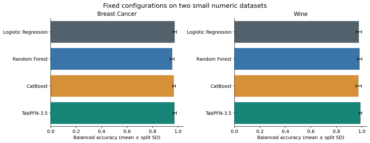
Now that all four models are available, we can compare their predictions. Our main metric is balanced accuracy. We calculate the share of correct predictions within each class, then average those shares. This gives each class equal weight.
We also record accuracy and macro F1. F1 combines precision and recall; the macro average gives each class equal weight. Log loss evaluates the probabilities and penalizes confident mistakes, so a lower value is better.
The notebook includes ROC AUC as well. For Breast Cancer, class 1 is benign and is treated as the positive class for binary AUC. Wine uses macro one-vs-rest AUC. All class predictions come from the largest predicted probability.
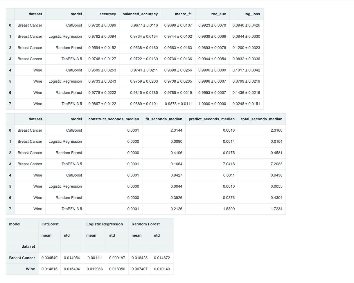
For the main comparison below, we focus on accuracy, balanced accuracy, macro F1, and log loss. The tables show the mean and sample standard deviation across five splits. Because the test sets overlap, the standard deviations describe the variation we observed. They aren’t confidence intervals or proof that one model will perform better on another dataset.
Breast Cancer Wisconsin

For Breast Cancer, Logistic Regression has the highest average balanced accuracy. Its difference from TabPFN is about 0.11 percentage points. I wouldn’t make much of that gap on these splits. TabPFN beats Logistic Regression twice, loses twice, and ties once when we compare the matching splits.
Logistic Regression has the better average class prediction scores here, while TabPFN has a slightly lower log loss. That distinction matters if we plan to use the probabilities. Predicting the correct class and assigning a good probability aren’t the same thing.
Wine

Moving to Wine changes the ranking. Here, TabPFN performs better across the four reported metrics. Its balanced accuracy is about 0.74 percentage points above Random Forest, the next model on that metric. On matching splits, TabPFN beats Random Forest twice and ties it three times.
The probability results give us another reason to consider TabPFN here. Random Forest ranks second on balanced accuracy but last on log loss, while TabPFN has the lowest log loss. If we only checked class predictions, we would miss this difference.
I would consider this a good result for TabPFN under these settings. I’d still want to see whether the improvement holds on a larger test set.
Alongside these summaries, we save the probabilities for every test row. This lets us inspect the predictions behind a score difference on the same rows. Prediction quality is only one part of choosing a model, though, so we also need to look at how long those predictions take.
How long do the models take?
To measure that time, I ran all four models on an Intel Core i7-12700H CPU with four compute threads. TabPFN uses one preprocessing worker. The notebook records the full environment, including Windows and Python 3.11.5.
Before timing the comparison, we run each model on a small subset. Then every measured run creates a fresh estimator, fits it, and predicts probabilities for the full test batch.
These timings start after package imports and the first weight download. Loading TabPFN’s cached weights stays inside the fit measurement, so the results include that work. The table below separates fit and prediction time to show where each model spends its time.
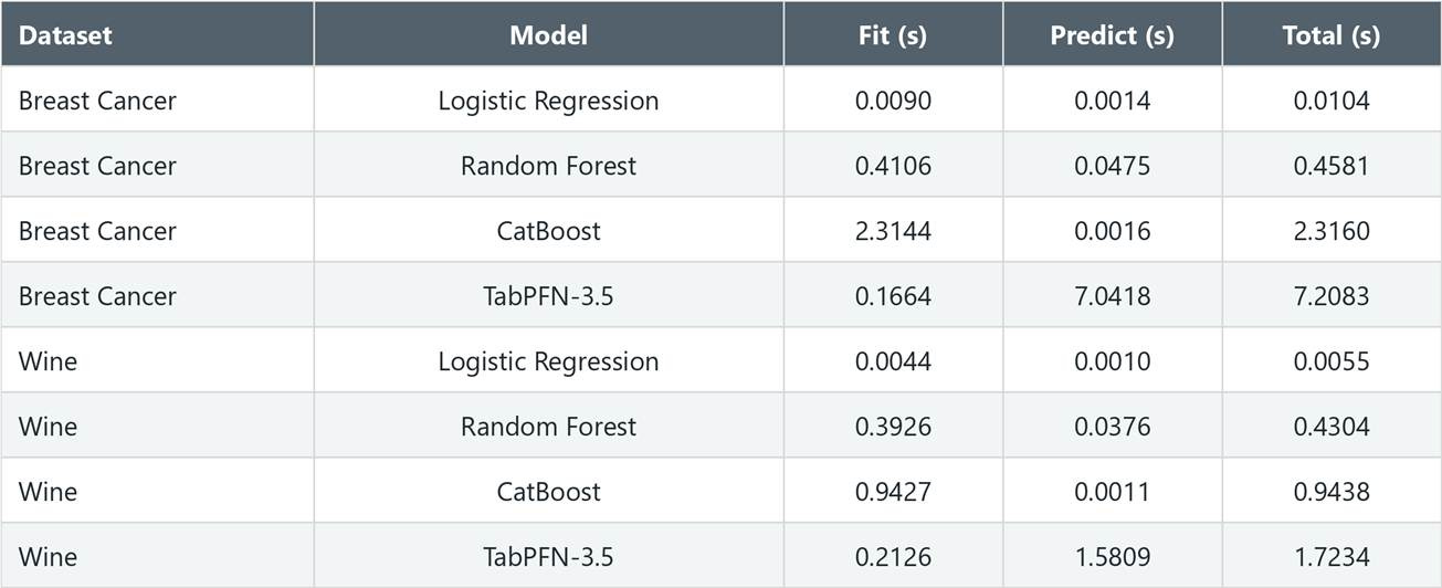
The part I would pay attention to is TabPFN’s prediction time. Most of its total runtime comes after fit(). Timing fit alone would leave out most of the work in this experiment.
Logistic Regression finishes fastest on both datasets, while TabPFN takes the longest total time. For a small offline analysis, waiting a few seconds might be acceptable. If we need to repeat the process many times, I would check whether the prediction improvement is worth that extra time.
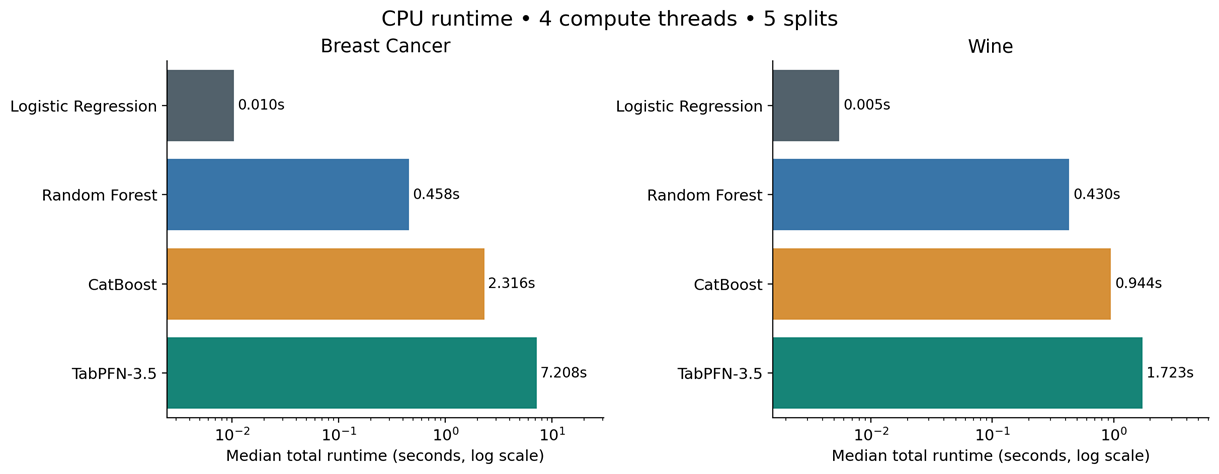
Image by the author. Total runtime uses a logarithmic axis.
When reading this chart, remember that we timed the first full-test prediction from a fresh estimator on the CPU after a separate warmup. These measurements don’t cover GPU performance or repeated predictions from a model kept in memory. A batch time also doesn’t tell us the response time for one request in a production service. We can review the measured scores and timings together in the notebook output below.
What would I use?
Taking the prediction scores and runtime together, I would still start with Logistic Regression for these small numeric datasets. It gives us strong scores with very little runtime, so I would run it before deciding whether we need another model.
I would include TabPFN in the comparison too. The Wine result gives us a reason to test it, especially when we care about the predicted probabilities. It doesn’t give us a reason to assume it will perform better on every table.
To see why those probability scores matter, imagine we’re using predictions to decide which records to review first. I would compare the probability scores and inspect the mistakes alongside runtime. If our task needs frequent predictions, the extra computation could change which model I choose.
For the same reason, I would keep Random Forest and CatBoost in the comparison when testing our own data. We used fixed settings here, and neither dataset tells us how the models compare when categorical features or tuning matter. Those gaps bring us to the limits of this experiment.
Where this comparison is limited
The first limitation is the amount of test data. There are only 45 Wine test rows in each split. A few changed predictions can affect the ranking, and our five overlapping holdouts aren’t independent experiments. I’d want to test more data before treating the Wine result as a reason to replace another model.
We also haven’t tuned the models. To extend this comparison, we could search within the training data and record the search budget for each model. The test labels should stay out of those choices.
Beyond tuning, the data itself needs a broader comparison. Both datasets are complete numeric tables, so we haven’t tested missing values or categorical features. We also haven’t measured larger datasets or peak memory. Any of these could change which model works best for our task.
Extending the experiment also means choosing a split that matches our data. For records ordered by time or connected through customers, we’d need a time-based or group-based split. Random splitting could put closely related records in both training and testing.

Conclusion
In this article, we compared TabPFN-3.5 with Logistic Regression, Random Forest, and CatBoost on two datasets using the same five train/test splits. We measured prediction performance and CPU runtime, then discussed the comparison’s limitations.
TabPFN led on Wine’s balanced accuracy and had the lowest log loss on both datasets. Logistic Regression was slightly ahead on Breast Cancer’s balanced accuracy and was much faster. These results show why we need to consider both prediction quality and runtime.
I would include TabPFN alongside traditional models when testing our own data. The comparison notebook and Python code provide a starting point for finding which model suits our task.
Continue Learning with Non-Brand Data
If you are interested in learning more about Data Science, Machine Learning, and AI, you can subscribe to Non-Brand Data. I regularly share articles, experiments, and examples that we can learn from.
For readers who want to explore a subject in more detail, the paid subscription also includes in-depth tutorials, written courses, notebooks, code, and additional learning materials.
I also offer 1-on-1 mentorship through MentorCruise if you want to discuss your learning direction, Data Science projects, technical challenges, or career development.