Elevate Your Jupyter Notebook Environment Experience

And subsequently, make you love to work in Jupyter Environment

And subsequently, make you love to work in the Jupyter Environment

Jupyter Notebook in the vanilla form

Jupyter Notebook is an inseparable part of me as a Data Scientist. Jupyter Notebook capable of testing my code in a different cell, showing my figure instantly, and even writing the necessary explanation in markdown form; an experience which not available in any other IDE (or as far as I know).

While I said that, I realize that Jupyter Notebook is more a tool for exploration and testing rather than for production. I also know that in their default form it could be painful to be used, especially for people who came from other IDE. Nevertheless, I want to show some features that I love from Jupyter Notebook to elevate our experience in using Jupyter Notebook. Just a little note, most of the extension here is only working properly by assuming the language that you use for your jupyter notebook is Python.

Here I create the part 2 of the article as an additional article to elevate your Jupyter notebook experience.

Markdown and LaTeX

For those who did not know what Markdown is, it is a language that adding formatting elements to the plain text document. Markdown gives you the versatility to manipulate your plain text into a much more interesting text (e.g. embedding link, image, or even video)

How Markdown Work

To use the markdown, we need to switch our cell into the markdown mode. We just need to select the Markdown selection from the drop-down. If you want to learn all the command used in the markdown format, you could learn it here.

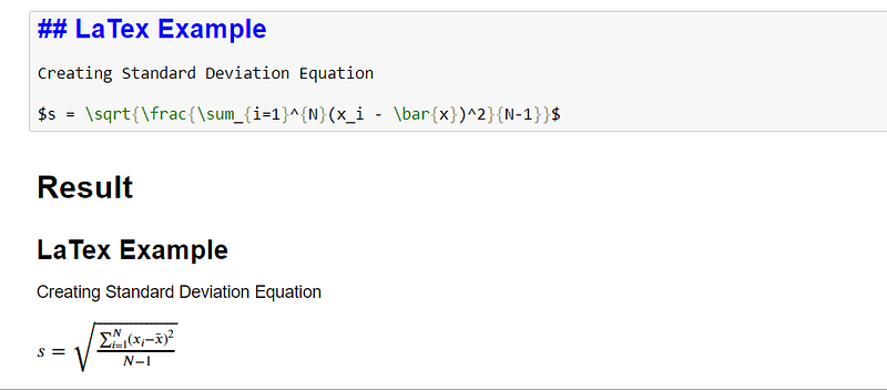
What I love about Markdown in the Jupyter Notebook is not the formatting part but how it actually could implement LaTeX in their cell. LaTeX is also a form of plain text formatting language. Specifically, it is often used for complex math expressions.

Standard Deviation Equation via LatEx in the Markdown cell

Just like Markdown, LaTeX has its own rule. If you want to learn more about it, there is an open-source guide for the LaTeX documentation here.

Programming Language Extension

When we install the jupyter notebook via Anaconda we would only be using Python as our working language. This creates an assumption that the jupyter notebook could only work with the Python language and we should use another IDE if we want to work with another language such as R or Julia. This is not true at all; we could implement other languages in our jupyter environment.

Jupyter notebook kernel selection

For example, we could embed an additional extension for our jupyter notebook environment to work with R or Julia programming language.

1. R Notebook

To have the R notebook in our jupyter notebook, we need to follow these steps:

1. Install R; We need to have our R programming language before we could set up R in our jupyter notebook environment. You could download it here.

2. Install IRkernel; IRkernel is a jupyter kernel that processing R language in the jupyter notebook. You could install the IRkernel via R console by typing install.packages('IRkernel').

3. Enable the IRKernel; For jupyter to see the newly installed IRkernel, we need to enable it via R console by typing IRkernel::installspec(user = FALSE).

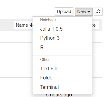
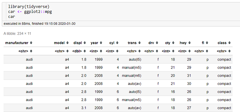
Now we could utilize the R programming language in our jupyter notebook by selecting the R when we create a new notebook.

R in Jupyter

2. Julia Notebook

How about Julia? Yes, we could also set up the Julia language in our jupyter notebook. We just need to follow steps similar to above.

1. Install Julia; Just like R, we need to download the Julia language as our first step. You could download Julia here.

2. Install IJulia; IJulia is the equivalent of IRkernel in R. We installing the IJulia by typing following line in the Julia command line:

using PkgPkg.add("IJulia")

Just like that, we now could use the Julia language in our jupyter notebook.

Julia in jupyter

Jupyter Notebook Extension

Jupyter Notebook contains an add-on or extension to improve our productibility. Will Koehrsen has created a great post on how to enabling this extension, but here I would summarize the installation part and show some of my favorite extensions.

To enabling our Jupyter Notebook Extension for the Python environment, we only need to run the following command in the terminal:

pip install jupyter_contrib_nbextensions && jupyter contrib nbextension install

The Jupyter extension tab

Opening the tab would present us with a great selection of extension shown below.

There are many extensions selections that the usefulness is depending on what kind of work we are doing, but I would show some that I often used.

1. Execute Time

I find Execute Time extension useful as I often testing various combinations of code to find the fastest one to run. The extension would show up every time we run the current cell and would remain there until we run the cell once more or resetting the notebook. Let me show it with an example below.

Execute Time Extension

When we have finished running the code, this extension would provide us with the code execution running time with the finish time.

2. Variable Inspector

One of the reasons why people did not like to use Jupyter Notebook is their lack of variable inspector which provided in another IDE. For that case, we have another extension called Variable Inspector.

How variable inspector work

Just what their name implies, these extensions would create an additional instance to show all the variables present in our jupyter notebook environment.

3. Code Prettify

With one push of a button, this extension would re-structured our codes. I often use this extension after a long process of coding to create a readable and neater line of codes.

This extension would not always work as we want. For example, if we already have a neat line then it would not change our line at all.

4. Scratchpad

This extension would create a stand-alone environment like a scratchpad in our book. Scratchpad is a really useful extension if we need a place for code experiments but did not want to interrupt our current jupyter environment.

Scratchpad example, red circle indicate the place to pop up the scratchpad

Supporting Package

Many modules have been developed to create a much seamless and interactive way to work with our data in the Jupyter environment. With time, I am sure this list of the modules would be developed even more, but here I would show some of the packages that I used daily.

1. Progress Bar

Most of the time, we take so much time to do our looping process but we do not even know when it would be finished. Moreover, we want to know if our looping is running properly or not.

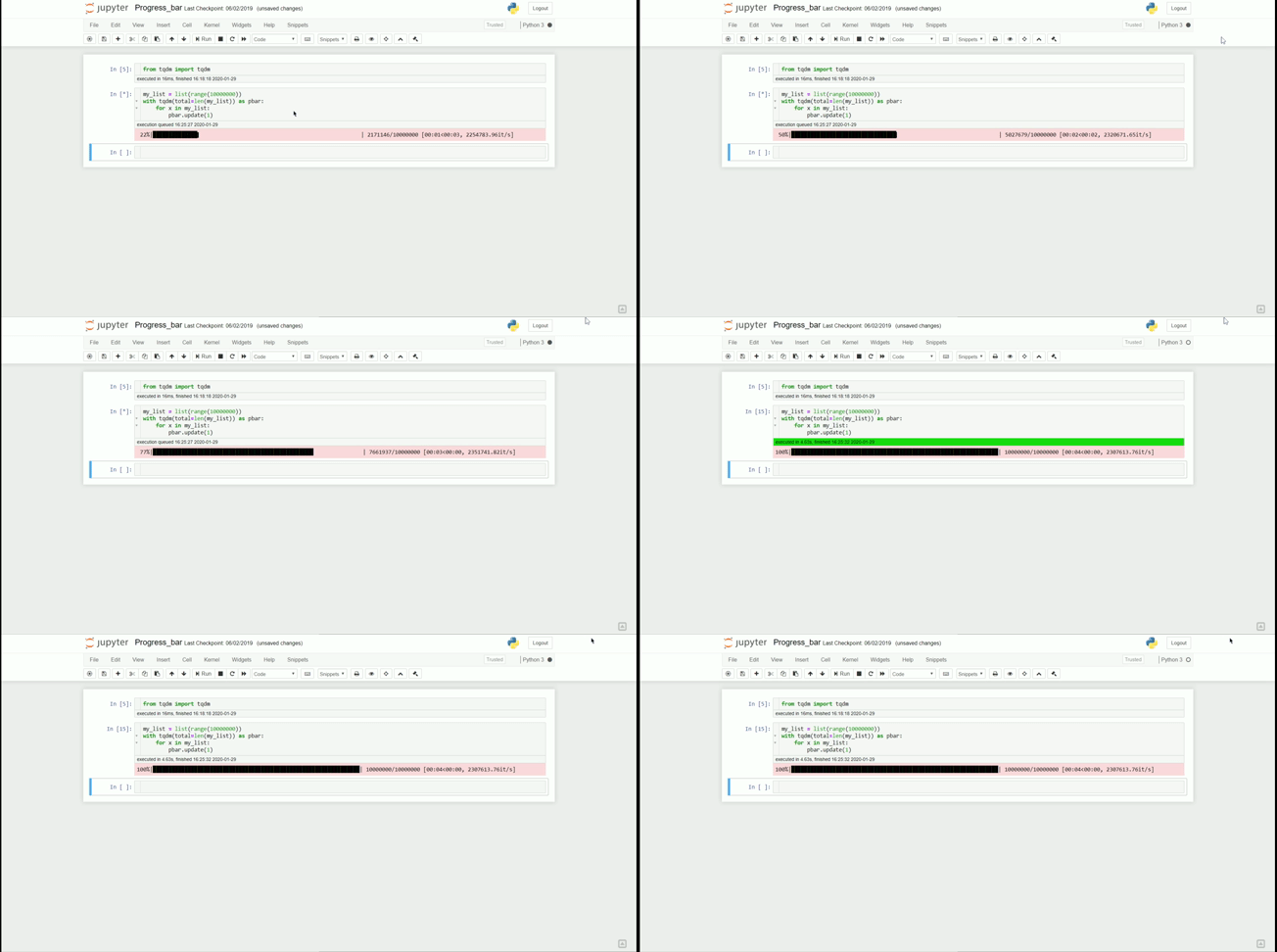
In that case, we could have a progress bar provided by the tqdm module. Below is an example of the progress bar in our jupyter notebook.

Progress Bar during looping session

We install the tqdm package by using pip or conda in our respective environment.

pip install tqdm

Below is the code example of how to add a progress bar in our jupyter notebook.

#Import the modulefrom tqdm import tqdm

#Creating the list for looping purposesmy_list = list(range(10000000))

#Calling the progress bar in the jupyter noteboookwith tqdm(total=len(my_list)) as pbar:    for x in my_list:        pbar.update(1) #use this code to move our progress bar

We call the progress bar by calling the tqdm with the total parameter accepting the number of iteration happening. To move the progress bar, in every iteration that occurs we need to update the progress bar by using the pbar.update() method which accepts the increment number (Usually it would be 1).

2. Widgets

While we work to exploring our data, sometimes it would be a hassle to keep editing our code just to show that certain plot. This certainly would hinder our productibility and even waste some of our precious time.

Here I would show an example of interactive control with the purpose to change our input without additional code editing by using the ipywidgets module.

How ipywidgets could produce a variety of plot without editing our code

First, we install our module by using the usual pip or conda.

pip install ipywidgets

Then we enabling our ipywidget module by typing this following code in our command prompt:

jupyter nbextension enable --py widgetsnbextension

With the extension in place, we could now activate interactive control in the jupyter notebook. Here is the code example from my GIF above.

#Import all the important moduleimport matplotlib.pyplot as pltimport seaborn as snsfrom ipywidgets import interact

#load the example datasettitanic = sns.load_dataset('titanic')

The Titanic Dataset

Let’s say I am interested to see the mean of the fare grouped by every categorical group in the dataset. We could filter the data one by one but it would take much time and decrease our productibility. For that reason, we could use the interactive control.

#Creating the interactive control

@interactdef create_fare_plot(col = titanic.drop(['fare', 'age'], axis =1).columns):    sns.barplot(data = titanic, x = col, y ='fare')    plt.title(f'Mean Bar Plot of the Fare grouped by the {col}')

We initiate the interaction with the ‘@interact’ code line, followed by the def statement to create the interactive control we want. Here the interact widget would give us the dropdown with the option from what we input in the def parameter.

Dropdown with all the categorical variable to switch between plot

Conclusion

Above is some example to elevate our experience in the jupyter notebook. I know that the jupyter notebook would never change IDE such as the Visual Studio Code for production purpose but I try to show how to improve the jupyter environment for Data Scientist work purposes.