Estimate the Causal Effect Intervention on Time Series with causalimpact
Infer the causal intervention effect on your Time Series Data
Infer the causal intervention effect on your Time Series Data

Imagine working as a Data Scientist in a company that sold candies, and the sales department in your company request help regarding their newest campaign. The Sales department wants to know whether their new campaign help to boost the company revenue or not in the long run, but because the cost of the campaign is expensive, they are unable to do any A/B testing; which means you only have the current experiment data to validate the real-world impact. What approach should we take?
There are few alternatives to solve this problem, e.g., descriptive revenue comparison before and after the campaign or experimental hypothesis testing. These methods are all viable but cannot measure the actual impact because many features affect the outcomes.
To solve this problem, the team at Google has developed an open-source package, Causal Impact on R, using Bayesian Structural Time Series. The Causal Impact package also available in Python, which we would use later.
In this article, I want to outline how Causal Impact works and how this package helps us a Data Scientist.
Let’s get into it.
Causal Impact
Concept
The Causal Impact concept is to solve the problem if there is an impact of intervention or action on the time-series data. In real-world cases, there are many instances that the only data we have is the result of our experiment and not the data if we are not doing any experiment or intervention.
Let me show you what I mean in the passage above with a sample below.
Going back to our imagination before, when we have a new campaign to increase the company revenue, the only data we had would be the revenue after the campaign and not the revenue if the campaign is not happening.
There might be a change in the revenue after the campaign, but are we sure if this because of the campaign and not some other reasons? We did not have the data if the campaign did not happen, after all.
This is where Causal Impact could help us evaluate our assumption. The way Causal Impact approached the problem is by using the Bayesian Structural Time Series to fit a model that best explains the “pre-intervention” data (In our example is the data before the campaign happens). The best model is used in the “post-intervention” data (after the campaign) to forecast what would happen if the intervention never happen.
Causal Impact mentions that the model would assume that the response variable (the intended target, e.g., revenue) can be modeled by linear regression with other variables (“covariates” or X) that are not affected by the time intervention. For instance, in our example, we want to assess the effect of a campaign on the revenue, then its daily visits cannot be used as a covariate as visit number might be affected by the campaign.
The inferences to assess the causal impact would then based on the differences between the observed response to the predicted one, which yields the absolute and relative expected effect the intervention caused on data.
If I summarize the Causal Impact procedure in an image, it will show like the picture below.
Coding Example
We can try the Causal Impact analysis with dataset example. Let’s try it with the following codes.
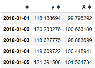
import numpy as npimport pandas as pdfrom statsmodels.tsa.arima_process import ArmaProcessfrom causalimpact import CausalImpact#Creating Random Generated time datanp.random.seed(12345)ar = np.r_[1, 0.9]ma = np.array([1])arma_process = ArmaProcess(ar, ma)X = 100 + arma_process.generate_sample(nsample=100)y = 1.2 * X + np.random.normal(size=100)y[70:] += 5#Data Frame with time indexdata = pd.DataFrame({'y': y, 'X': X}, columns=['y', 'X'])dated_data = data.set_index(pd.date_range(start='20180101', periods=len(data)))#Time period for pre-intervention and post-interventionpre_period = ['20180101', '20180311']post_period = ['20180312', '20180410']dated_data.head()Right now, we have a Data Frame with two columns, y and X. Using the Causal Impact, your intended target to assess should be renamed as y, and the other columns would be treated as the covariate feature.
To separate the time intended as the pre-intervention data and post-intervention data, you should set the index of your data using the DateTime object and create two lists consisting of the time range (both for pre-and post-intervention).
Let’s try using all this information for the Causal Impact analysis.
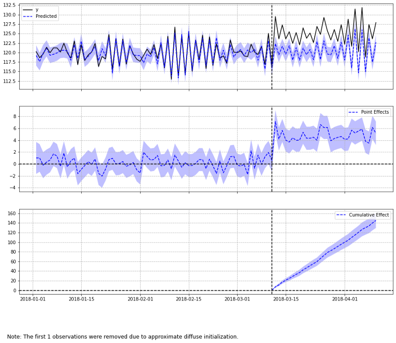
#Using Causal Impact analysis, the three parameter you should fill (data, pre-intervention time, post-intervention time)ci = CausalImpact(dated_data, pre_period, post_period)ci.plot()When we plot the results, there are three plots as a default output:
The top part which is the original series versus its predicted one
2. The middle part, which is the points effects plot; the difference between the original series and the predicted
3. The bottom part is the cumulative effect plot. This is the summation of the point effects accumulated over time.
If you are not sure what the plot is telling us, we can see an increasing effect because of the time intervention event by looking at the cumulative effect.
For consideration, Causal Impact recommends that we set the prior parameter as None just like the following code to let the model do all the optimization.
#Add prior_level parameterci = CausalImpact(dated_data, pre_period, post_period, prior_level_sd=None)ci.plot()If you want to see all the Causal Impact's statistical results, you can run the following code.
print(ci.summary())For the example above, we can see that the absolute effect is 4.78, where the predictions could vary from 4.17 to 5.38 with a 95% confidence interval. This means there is an increase of 4.78 units with intervention happens. Although, don’t forget to check the p-value before making any conclusion.
If you need more elaborate results, you could run the report summary code.
print(ci.summary(output='report'))In this case, you would obtain all the information regarding the effect of the time intervention.
In the case you need deeper analysis, you could run this code to acquire the information of the prediction for each time point.
ci.inferences.head()Here all the predicted information is summarized into one data frame object. You could create your own visualization if you want to play around with this data.
Additionally, if you want to analyze the model, you could run this code.
ci.trained_model.paramsYou might want to evaluate the model parameter if you feel the parameter cannot help the model predict the response variable.
Conclusion
As a Data Scientist, we might need to assess an event's effect on the time-series data. While it is possible to evaluate it using a simple statistic, the challenging part is to confirm whether the event actually affects the result.
In this case, we could use an analysis called Causal Impact to address the impact problem. This package is easy to use and produces all the results to support your hypothesis if intervention affects the response variable.


