Estimating Time until Contract Termination — Survival Analysis with Lifelines

Estimating the time for a particular event occurring with Lifelines

Feb 08, 2021

I am sure everyone at some point of their data career would meet a case when you want to estimate a specific event to happen, e.g., “When someone would churn?” or “When the death claim of insurance would happen?”. We would commonly use a time-series approach to solve this problem, but Survival Analysis is the typical approach.

In this article, I want to introduce to you what is Survival Analysis and its application with the Lifelines Python package using real-life Contract Termination data. Let’s get into it.

Survival Analysis

Introduction

What is Survival Analysis? Survival analysis is a statistical analysis developed to measure individuals' lifespans; for example, “how long does this population live for?”. This would be answered using the survival analysis.

While initially it is used to measure individual lifespan (life or death), the analysis is versatile enough to answer all kinds of questions. You might be interested in the time between people buying the insurance until the time of the claim or when people come into the theme park until they are exiting the park. What is important is the data have the duration of the event.

Censoring

You might have a follow-up question after my explanation above “I might have the data, but what if I did not have all the data with the duration of the event I want.” For example, you might need to wait until 60 years until all the individuals you analyze claim their death insurance — but you want to decide in a time faster than that (possibly right now).

This is why we have the right-censored concept. The concept defines the individual with the non-occurring event lifetime (or duration) excluded, and the only information we had is the current duration.

To clarify, we would use a dataset example from Kaggle regarding the Employment Attrition where their contract is terminated.

import pandas as pddf = pd.read_csv('MFG10YearTerminationData.csv') df[['length_of_service', 'STATUS']]

We might ask this question from the data “What is the duration of the time until employee contracts are terminated?”. As we are interested in the termination time, we need the employee data with their contract status (ACTIVE or TERMINATED).

If you see the data above, we would have the length_of_service. This is the time in months of the employee serving within the company until now or until their contract is terminated. If the status is still ACTIVE, then we have right-censored the data as we still did not know when their employment contract would be terminated (we put the length_of_service for the ACTIVE status with the months between their hired time until the current time).

The censoring is also done to alleviate the problem of different times of entering for some individuals. The data we have would certainly not have the employee hired simultaneously; some are employed a long time ago, and some are a recent addition.

Why do we need to know about right-censored? This is because Survival Analysis is developed to deal with the estimation using the right-censored data. All our estimates would be based on the data we right-censored.

If you are still not comfortable with the concept, let’s get into the application using the Lifelines Python package.

Lifelines

I would skip the Survival Analysis mathematical part as the central part of this article is to use the Lifeline package to estimate the time until the contract termination. If you are interested in an in-depth math explanation of the Survival Analysis, you could visit the Lifeline package here.

Installation

For the preparation, let’s install the Lifelines package.

#install with pippip install lifelines

#install via condaconda install -c conda-forge lifelines

Survival Function with Kaplan-Meier Estimation

With the package installed, we are now ready to do our Survival Analysis with the Lifelines package. As a starter, we would estimate the Survival Function using the Kaplan-Meier estimation.

from lifelines import KaplanMeierFitterkmf = KaplanMeierFitter()

While the dataset is ready, we would do one feature engineering to transform the ‘STATUS’ variable into 0 or 1 instead of text (This feature would be called ‘Observed’).

df['Observed'] = df['STATUS'].apply(lambda x: 1 if x == 'TERMINATED' else 0)

Now we have all the data we need; the duration and the event observed. Let’s start by creating the Survival Function.

#Kaplan-Meier estimationkmf.fit(df['length_of_service'], df['Observed'])

If it is successful, this notification will show up in your notebook.

Next, we could try to plot the survival function to see the survival probability (probability of employee contract termination is not happening) throughout the time.

import matplotlib.pyplot as pltplt.figure(figsize = (8,8))plt.title('Employee Contract Termination Survival Function')kmf.plot_survival_function()

The plot above shows the probability of the employment contract would not terminate following the time. The plot showing interesting information; during the first 23 months, the likelihood of your contract terminated is relatively low, but when you are entering the 24 months and 25 months, your survival probability (contract not terminated) becomes significantly lowered. This means that most of the termination happens in the month 24 or 25 of your contract times.

If you are more interested in the actual number than the plot shows, you can show the survival function estimation by running the following code.

kmf.survival_function_

Or, if you are more interested in the cumulative density of the termination probability, you could run the following code.

kmf.cumulative_density_

Comparing two different Kaplan-Meier Estimation

We might have another question; “Is there a contract termination time difference between the gender?”. To answering this question, we could set up two different datasets and survival functions.

#Separate the Male and Female datadf_m = df[df['gender_short'] == 'M']df_f = df[df['gender_short'] == 'F']

#Prepare the survival functionkmf_m = KaplanMeierFitter()kmf_f = KaplanMeierFitter()

#Estimate both dataset to acquire the survival functionkmf_m.fit(df_m['length_of_service'], df_m['Observed'], label = 'Male')kmf_f.fit(df_f['length_of_service'], df_f['Observed'], label = 'Female')

#Produce the survival function plotplt.figure(figsize = (8,8))plt.title('Employee Contract Termination Survival Function based on Gender')kmf_m.plot_survival_function()kmf_f.plot_survival_function()

Here we have another exciting result. The plot shows that the survival probability for the Female is way lower than the Male. In month 25, we have a significant survival probability drop for the females compared to the males.

We can use statistical hypothesis testing to assess our assumption if there is a difference between males and females for their contract termination time. The standard test to use is the log-rank test, which Lifelines provide within the package.

from lifelines.statistics import logrank_test

results = logrank_test(df_m['length_of_service'], df_f['length_of_service'], df_m['Observed'], df_f['Observed'], alpha=.95)

results.print_summary()

From the test result, we acquired P-value less than 0.05, which means we reject the Null Hypothesis and accepting that there is a difference between males and females in their contract termination time. It is a disturbing thing but let’s put aside the conclusion until we analyze things even further.

Hazard Function using Nelson-Aalen

Previously we talk about the survival function, but you might be more interested in the probability of death (contract termination) event happening at the time of t. Itis what the Hazard function was about, estimating the probability of death.

We would use the Nelson-Aalen estimation as the way to estimate the Hazard Function. Luckily, the lifelines packages have provided this function.

from lifelines import NelsonAalenFitternaf = NelsonAalenFitter()

naf.fit(df['length_of_service'], df['Observed'])plt.figure(figsize = (8,8))plt.title('Employee Contract Termination Hazard Function')naf.plot_cumulative_hazard()

The Hazard function feels like the reverse of the Survival function. From the plot, we can see that it starts slow and going high at the end in the month 24 and 25. Although, what you see here in this plot is the cumulative hazard rate, and we interpret the result by looking at the rate at the time t.

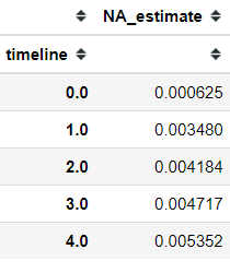
If we want to get the actual number of times t, you could run the following code.

naf.cumulative_hazard_

Cumulatively, the hazard rate would get higher as the time probability of contract termination event happening is increasing following the time.

Survival Regression with Cox’s proportional hazard model

Often, you would have another data other than the duration you assume would affect the Survival analysis. This technique is what we called the Survival Regression.

There are a few popular models in survival regression, but Cox's model is most commonly used for this problem. Let’s try this model with the dataset we own before.

I assume that only Age, Gender, and Business Unit affects the duration of the employee contracts.

training = df[['age', 'gender_short', 'BUSINESS_UNIT', 'length_of_service','Observed']].copy()

From this data, we need to prepare it to be Machine Learning ready. It means we need to One-Hot Encode the categorical variable.

training = pd.get_dummies(data = training, columns = ['gender_short', 'BUSINESS_UNIT'], drop_first = True)

training.head()

This is the dataset that we would use for Cox’s model. Let’s see if these variables are affecting the employee contract termination time.

from lifelines import CoxPHFitter

cph = CoxPHFitter()cph.fit(training, duration_col='length_of_service', event_col='Observed')cph.print_summary()

From the model summary above, we can see that the BUSINESS_UNIT_STORES is the only variable that did not affect the duration because the P-value is more than 0.05 while the rest has a significant result.

For the interpretation, we can assess the coefficient of the variable. Let’s take the age coefficient, which is -0.01. It means, one unit of increase in the age would decrease the baseline hazard function by exp(-0.01) or 0.99. You could interpret this by saying that with an increase in age, the chance of contract termination would decrease by around ~1%.

After fitting the model, we can use this model to predict the new data's survival function.

cph.predict_survival_function(training[['age', 'gender_short_M', 'BUSINESS_UNIT_STORES']].loc[0]).plot()

The data we give to the model produce us this following survival function where the probability of the survival would decrease significantly on the month 25 (around ~50%).

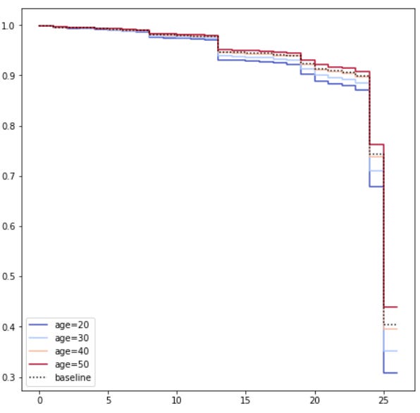
To understand the model even better, we can plot the survival curves to look like we vary a single variable while holding everything else equal. This is used to understand the impact of the variable given the model we had.

We want to understand the age variable impact on our model; we can plot using the following code.

cph.plot_partial_effects_on_outcome(covariates='age', values=[20,30, 40, 50], cmap='coolwarm', figsize = (8,8))

Given the age, we can see that the survival probability increases with the increase of age. This means we can assume that older people are less likely to have their contract terminated than younger people.

Conclusion

Survival Analysis is an analysis that tries to solve a problem with a question such as “When someone would churn?” or “When the death claim of insurance would happen?”.

Using the Lifeline package, we could do Survival Analysis easier, as we can see from the Contract Termination data. Using the Survival Analysis, we found out that the probability of someone would have their contract terminated is the highest when the employee is reaching 24 and 25 months of their working time. Moreover, females and younger people having a higher probability of having their contract terminated.

Non-Brand Data

Discussion about this post