Fantastic Pandas Data Frame Report with Pandas Profiling

Enhance your basic reporting to the next level

Enhance your basic reporting to the next level

Source: Created by Author

As a Data Scientist, we would explore data for our everyday work. For Pythonist, using the Pandas module is a must. While compelling, sometimes we find the report is just too basic. Let me show it by an example below.

import pandas as pdimport seaborn as sns

#Loading dataset mpg = sns.load_dataset('mpg')mpg.describe()

We could produce the fundamental statistic using .describe() attribute, but instead of a basic report like the sample above, we could have our report way more attractive like below.

Just look at how different the report becomes. It makes our daily exploration way easier. Furthermore, you could save the report into HTML and share it with anybody you want. Let’s just get into it.

Pandas Profiling

We could create a fantastic report like above with the help of Pandas Profiling module. This module is the best to work in the Jupyter environment so that this article would cover the report generated in the Jupyter Notebook. Now, to use this module, we need to install the module.

#Installing via pippip install -U pandas-profiling[notebook]

#Enable the widget extension in Jupyterjupyter nbextension enable --py widgetsnbextension

#or if you prefer via Condaconda env create -n pandas-profilingconda activate pandas-profilingconda install -c conda-forge pandas-profiling

#or if you prefer installing directly from the sourcepip install https://github.com/pandas-profiling/pandas-profiling/archive/master.zip

#in any case, if the code raise an error, it probably need permission from user. To do that, add --user in the end of the line.

With that, we are ready to generate the report. We would use the Pandas Profiling function, just like the code below.

#Importing the functionfrom pandas_profiling import ProfileReport

#Generate the report. We would use the mpg dataset as sample, title parameter for naming our report, and explorative parameter set to True for Deeper exploration.

profile = ProfileReport(mpg, title='MPG Pandas Profiling Report', explorative = True)

profile

After waiting a while, we would end up with an HTML report like below.

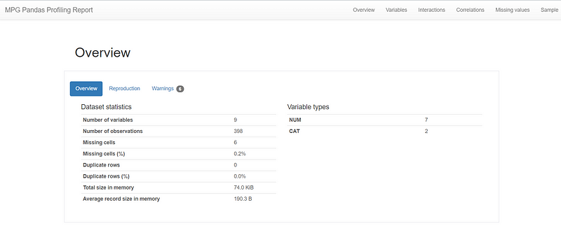
In the first part, we would get the overview information of our Data Frame. It is similar if we use the.info() attribute from the Pandas Data Frame object, but the Pandas Profiling offer more information. For example, the Warnings section.

What is excellent about the Warnings section is that the information given are not just basic info such as missing data, but more complex one such as high correlation, high cardinality, etc. We could modify how high it is to consider what is ‘High Cardinal’ or ‘High Correlation’, but I would not discuss it in this article.

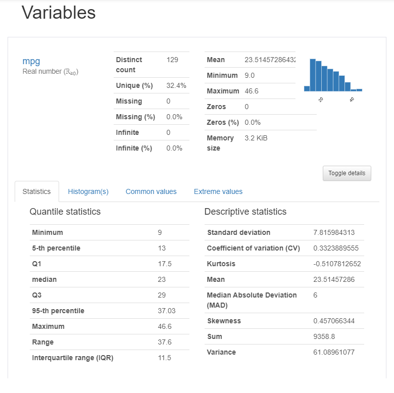
If we scroll down, we would see the Variables Section, which shown all the Numerical and Categorical columns with more detail. Below is the example of the numerical variable.

We could see that for each variable, we are served with complete statistic information. Furthermore, there are sections where we could get information for the most common values and extreme values.

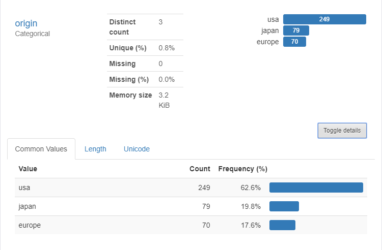
How about Categorical variable? Let me show you in the image below.

Just like the numerical variable, we acquired complete information about the variable. Scroll down even further; we would arrive in the Interactions section. This is the section where we could get a Scatter Plot between two numerical variables.

And just below it is the Correlations section.

This section is showing the correlation values between numerical variables in the form of a heatmap. Only four correlation calculation available here and if you need the correlation descriptions, you could click the “Toggle correlation descriptions button”.

There is also a section dedicated to the Missing values, just like the example below.

And the last section would only show the data samples — nothing interesting there.

If you need a more simple way to show the report, we could use the following code to transform the report.

profile.to_widgets()

With one line of code, we get the same information from what I showed you above. The only differences are just the UI becomes more straightforward. The information, although, would still the same.

Lastly, if you want to export the report into an external HTML file, we could use the following code.

profile.to_file('your_report_name.html')

You could find the HTML file in the same folder with your Jupyter Notebook. If you open the file, it would automatically open on your default browser with beautiful UI similar to the one in our Jupyter Notebook.

Conclusion

I have shown you how to transform our basic report in the Pandas Data Frame to a more interactive form by using the Pandas Profiling Module. I hope it helps.