

Time-series forecasting helps us estimate future values so we can plan ahead. For example, we can use historical sales data to predict demand and decide how much inventory to prepare for the coming month. We look for patterns in observations collected over time and use them to make these estimates.
For this task, we can try TimesFM-3, a pretrained forecasting model from Google Research. It allows us to generate predictions without training a model from scratch.
In this article, we’ll learn how to use TimesFM-3 for time-series forecasting in Python. Let’s get into it.
What Is TimesFM-3?
TimesFM-3 is a time-series foundation model developed by Google Research. We can provide historical observations and generate predictions with its pretrained weights. This approach is called zero-shot forecasting because we don’t train or fine-tune the model on our dataset.
Compared with earlier versions, TimesFM-3 adds native support for multivariate forecasting and covariates. Multivariate forecasting means predicting related time series together. Covariates are additional variables that can help the prediction, such as temperature or calendar information.
Some covariates are only available for past dates, while others are known in advance. For example, we have recorded temperatures for the past, but we can calculate weekend dates for the future. We’ll try both in our example.
Setting Up the Environment
First, download the code from the GitHub repository and install the required packages from the project folder:
python -m pip install -r requirements.txtWe’ll use the timesfm3 interface from the timesfm package. The repository includes the tested dependencies and setup instructions.
The downloadable model weights are licensed for non-commercial, non-production use, so check the license before using them for your project.
Preparing the Bike Sharing Dataset
For the dataset example, I use the UCI Bike Sharing dataset. It contains rental counts from Capital Bikeshare during 2011 and 2012, along with weather information. There are daily and hourly files, but we’ll use day.csv so each observation represents one day.
Let’s load the dataset and prepare the historical and test data with the following code:
import io
import urllib.request
import zipfile

import numpy as np
import pandas as pd
import matplotlib.pyplot as plt

url = "https://archive.ics.uci.edu/static/public/275/bike+sharing+dataset.zip"
with urllib.request.urlopen(url, timeout=60) as response:
    payload = response.read()

with zipfile.ZipFile(io.BytesIO(payload)) as archive:
    with archive.open("day.csv") as daily_file:
        df = pd.read_csv(daily_file, parse_dates=["dteday"])

df = df.sort_values("dteday").set_index("dteday")
assert df.index.is_unique
assert df.index.equals(
    pd.date_range(df.index.min(), df.index.max(), freq="D")
)
assert df[["cnt", "registered", "casual", "temp"]].notna().all().all()
assert (df["cnt"] == df["registered"] + df["casual"]).all()

horizon = 14
history = df.iloc[:-horizon].copy()
test = df.iloc[-horizon:].copy()
The code above sorts 731 daily observations by date and checks for missing or duplicate dates. We keep the final 14 days as test data and use the earlier observations as our history.
We’ll start with cnt, the total rental count, then try registered and casual rentals as related targets.
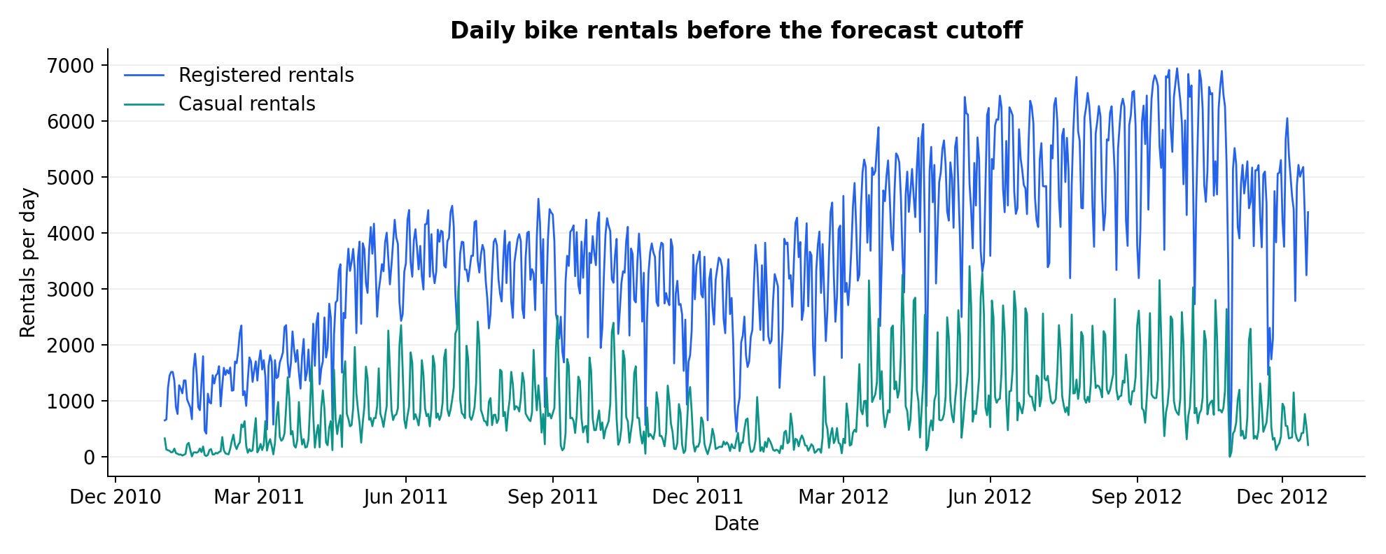
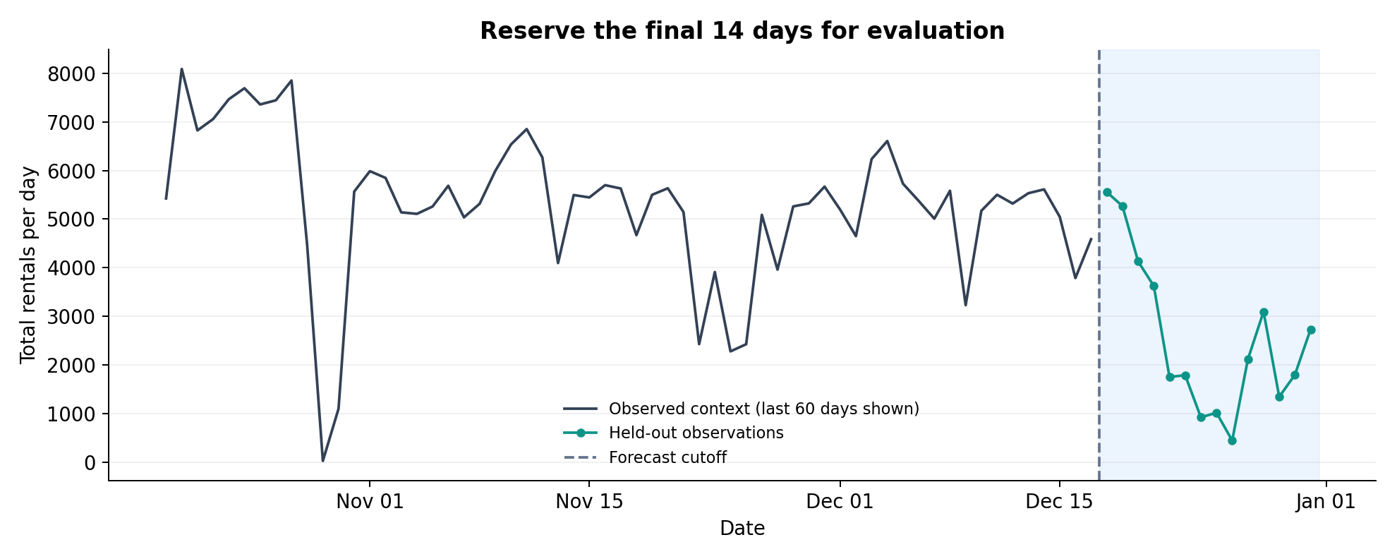
We split the data in date order so the model only receives observations from before the forecast period.
Generating Our First Forecast
With the dataset ready, let’s generate our first prediction using TimesFM3Forecaster:
from timesfm3 import TimesFM3Forecaster

forecaster = TimesFM3Forecaster.from_pretrained(
    "google/timesfm-3.0-pytorch"
)

context = history["cnt"].to_numpy(dtype=np.float32)
univariate = forecaster.predict(
    context=context,
    horizon=horizon,
    return_quantiles=True,
)
print(univariate.forecast.shape)   # (14,)
print(univariate.quantiles.shape)  # (14, 9)
In the code above, context contains the historical rental counts, and horizon sets the number of future steps. Since our observations are daily, horizon=14 gives us a two-week forecast.
The forecast attribute contains the predicted median for each day. With return_quantiles=True, we also get nine quantiles, from the 10th to the 90th percentile, to describe the model’s uncertainty.
Forecasting Multiple Variables
Next, let’s try the multivariate prediction with the same dataset. This time, we’ll predict registered and casual rentals together. We’ll also pass historical temperature and a weekend indicator using the following code:
future_dates = pd.date_range(
    history.index[-1] + pd.Timedelta(days=1),
    periods=horizon,
    freq="D",
)

targets = history[["registered", "casual"]].to_numpy(dtype=np.float32).T
past_temperature = history[["temp"]].to_numpy(dtype=np.float32).T

all_dates = history.index.append(future_dates)
weekend = (all_dates.dayofweek >= 5).astype(np.float32)[None, :]

multivariate = forecaster.predict(
    context=targets,
    horizon=horizon,
    past_only_covariates=past_temperature,
    past_future_covariates=weekend,
    return_quantiles=True,
)
print(multivariate.forecast.shape)   # (2, 14)
print(multivariate.quantiles.shape)  # (2, 14, 9)
Each row in targets represents a rental category, and each column represents a day. We use .T to arrange the data in this format.
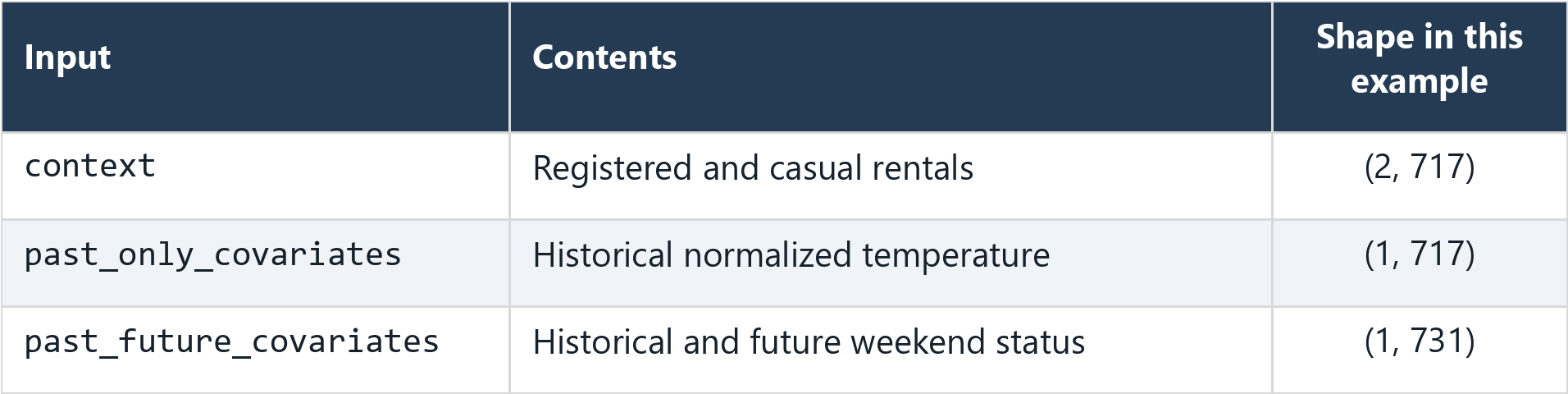
The historical inputs must refer to the same dates. The weekend array also covers the forecast period because we know those dates in advance.
We now have two sets of predictions, with registered rentals in the first row and casual rentals in the second.
We only provide historical temperature. Using the actual temperatures from the test period would introduce data leakage, as those measurements weren’t available when making the forecast. The weekend indicator is available in advance, but it doesn’t account for public holidays.
Visualizing and Evaluating the Results
To see the prediction result, let’s create a plot with the historical data and the actual values from our test period:
q = np.asarray(forecaster.config.quantiles)
lo = int(np.flatnonzero(np.isclose(q, 0.1))[0])
hi = int(np.flatnonzero(np.isclose(q, 0.9))[0])

fig, ax = plt.subplots(figsize=(10, 4))
ax.plot(history.index[-28:], history["cnt"].iloc[-28:], label="History")
ax.plot(future_dates, test["cnt"], "o-", label="Actual")
ax.plot(future_dates, univariate.forecast, label="TimesFM-3 median")
ax.fill_between(
    future_dates,
    univariate.quantiles[:, lo],
    univariate.quantiles[:, hi],
    alpha=0.2,
    label="10th-90th percentile band",
)
ax.set(ylabel="Rentals per day", xlabel="Date")
ax.legend()
fig.autofmt_xdate()
plt.show()
We can also plot registered and casual rentals and add a weekly baseline for comparison:
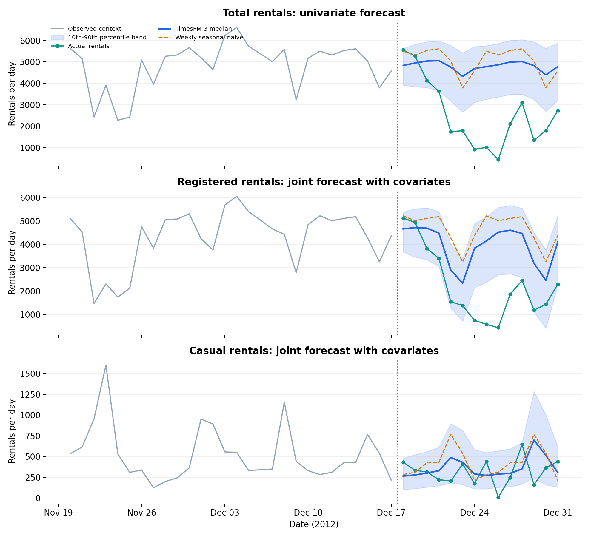
The shaded area shows the 10th–90th percentile band, a nominal 80% interval. Its actual coverage still needs to be evaluated.
To measure prediction error, we’ll use mean absolute error, or MAE. It calculates the average absolute difference between the predicted and actual values. A lower MAE means a smaller error.
Let’s compare the model with a seasonal naive baseline, which repeats the last observed week’s rental counts:
weekly_baseline = np.resize(
    history["cnt"].to_numpy()[-7:], horizon
)
actual = test["cnt"].to_numpy()

model_mae = np.mean(np.abs(actual - univariate.forecast))
baseline_mae = np.mean(np.abs(actual - weekly_baseline))
print(f"TimesFM-3 MAE: {model_mae:.2f}")
print(f"Weekly baseline MAE: {baseline_mae:.2f}")
The baseline repeats the same observed week twice, without using any values from the test period.
The results for all three targets are as follows:
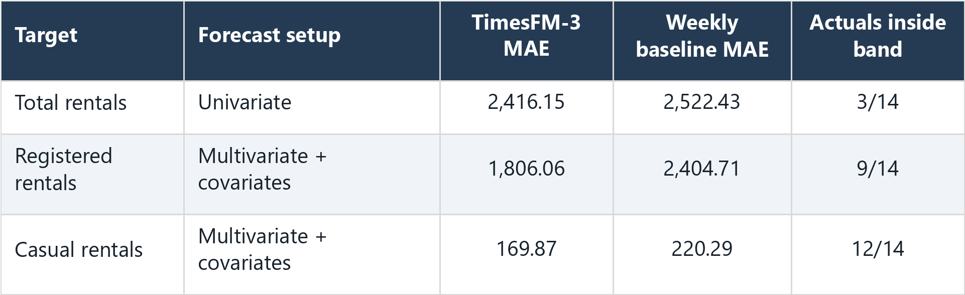
For this test period, TimesFM-3 has a lower MAE than the weekly baseline for all three targets. However, the total rental interval contains only three of the 14 actual values.
The total rental forecast still misses much of the decline toward the end of the test period. Its MAE is only 4.2% below the baseline’s error, so I wouldn’t call it reliable from this result alone.
Compare each target with its own baseline. Casual rentals have smaller counts, so their lower MAE doesn’t automatically mean a better forecast.
What Should We Know Before Using TimesFM-3?
Our example covers one forecast period. We should repeat the evaluation at several starting dates before deciding whether the model meets our needs. The joint example also changes the targets and adds covariates at the same time, so it doesn’t tell us how much each feature helps.
Zero-shot forecasting doesn’t guarantee that a dataset was absent from pretraining. The model card doesn’t confirm whether these bike rental records were included, so this example shouldn’t be treated as an unseen-data benchmark.
Keep the total rental forecast separate from the joint predictions. Adding the registered and casual medians or quantile bounds doesn’t generally produce the total’s median or a valid interval.
For a SQL alternative, TimesFM-3 is also available in BigQuery preview.
Conclusion
In this article, we learned how to use TimesFM-3 for time-series forecasting in Python. We started with daily bike rentals, then tried related targets and additional variables.
You can find the complete code in the GitHub repository.
I hope it helps!
Continue Learning with Non-Brand Data
If you are interested in learning more about Data Science, Machine Learning, and AI, you can subscribe to Non-Brand Data. I regularly share articles, experiments, and examples that we can learn from.
For readers who want to explore a subject in more detail, the paid subscription also includes in-depth tutorials, written courses, notebooks, code, and additional learning materials.
I also offer 1-on-1 mentorship through MentorCruise if you want to discuss your learning direction, Data Science projects, technical challenges, or career development.