Grimm’s Tales Topic Analysis via LDA: Why some Tales are Famous

Topic prediction study on the old tales

Nov 22, 2020

I am always a fan of fairy tales, and one of them is the Grimm Brother’s Tales collection. For you who don’t know about Grimm’s Tales, you might probably ever heard about Cinderella, Snow White, Red Riding Hood, Rapunzel, etc. Those tales are examples of fairy tales in the Grimm’s Tales.

Knowing some tales are famous and some are not, I am intrigued to know why some are more famous than others. I am assuming that tales are famous because of their story; that is why I commence this analysis; topic prediction analysis to pinpoint the famous topic.

Let’s get into it.

Latent Dirichlet Allocation (LDA)

Latent Dirichlet Allocation is an unsupervised analysis, which is not used to create a prediction model but rather a data mining technique. It was used to cluster words into similar groups.

LDA works by measures the probability distribution of topics belonging to the document. For example, if observations are words collected into documents, each document is a mixture of a small number of topics, and that each word’s presence is assigned to one of the document’s topics.

While it is interesting to know more about LDA, it would not be the main point of this article. I would create another article just for explaining LDA, but I know that LDA cluster the word for topic prediction analysis.

Data Preparation

For this analysis, I would use the data I scraped from the website here. If you want to have the cleaner version, I have put it in to Kaggle.

Let’s start by checking out the data we had and see what we can do with it.

import pandas as pddf = pd.read_csv('grimms_tales.csv')df.head()

The data we have consisted of four columns; Title (The Tales Title), Story (The complete story of the Tales), Rating (Rating Average from 0–10 voted by the viewer), and Voters (Number of votes).

For now, I would only consider the topic from the Story columns as I think that Story should be the one that decides why some Tales are famous.

For the sake of data modeling, let’s do some simple preprocessing. I would only do these three things; Lowering all the words, remove punctuation, and remove the stopwords. Let’s get into it.

from nltk.corpus import stopwords#if you have not download the stopwords yet# import nltk # Imports the library# nltk.download_shell() #Download the necessary datasetsimport string

#Creating the stopword list, I add some stopword I assume did not important

stopword = list(set(stopwords.words('english')))stopword.extend(['said', 'will', 'thou', 'did', 'went'])

#Creating the word cleaning functiondef word_clean(x):    nopunc = ''.join([char.lower() for char in x if char not in string.punctuation])    clean_mess = ' '.join([word for word in nopunc.split() if word.lower() not in stopwords.words('english')])    return clean_mess

df['Story_processed'] = df['Story'].apply(word_clean)df.head()

Now, we have added another column where the Story was cleaned up. Basically, we ended up with only the meaningful word of the story.

People who do Text analysis always do a word cloud, but I want to skip it right now because it is not the point of the article. Although, if you want to create a nice word cloud, you can check my other article.

Creating a Catchier Word Cloud Presentation
To get your audience’s attention better and your point deliveredtowardsdatascience.com

Modeling

The next step we would do is try the LDA modeling to create a word cluster for topic prediction. Let’s prepare everything we need.

First, we need to transform our text information into something that machine learning could accept (numerical information). In this case, we would create a bag of words.

For you who did not know a bag of words, the simpler explanation is that it was a count of the words within a document (in our case is the story). There are many functions already crated to create a bag of words, and we would use one of them.

#Class function to create a bag of wordsfrom sklearn.feature_extraction.text import CountVectorizer

There are many parameters we could set up in our CountVectorizer class, but there are four parameters that I would set up in our analysis; stop_words to set up the stop words, ngram_range to get the n-gram words that I want, min_df to set the words need to appear minimum times across the document, and max_df to limit the word that appears too much.

# Initialise the count vectorizer with the English stop words, and setting the parameter. This is an experimental one, but I set it too a minimum 5 and maximum frequency 0.8 to have a word that was not too rare but not too often.

count_vectorizer = CountVectorizer(stop_words='english', ngram_range=(1, 4), min_df = 5, max_df = 0.8 )

count_data = count_vectorizer.fit_transform(df['Story_processed'])

The code above would result in the sparse matrix of all the word count for each document. In the next step, we would proceed with the topic prediction using LDA.

LDA is an unsupervised analysis that assigns the probability of words in the topic and the topic's probability within a document. The LDA cannot measure the number of the topic in the corpus; because of that, we need to set it up on our own. However, we can use the grid search to help us with our case.

from sklearn.decomposition import LatentDirichletAllocation as LDAfrom sklearn.model_selection import GridSearchCV

# Define Search Paramsearch_params = {'n_components': [2, 3, 4, 5, 6,7,8,9,10, 15, 20, 25]}

# Init the modellda = LDA()

# Init Grid Search classmodel = GridSearchCV(lda, search_params)

#Fit the modelmodel.fit(count_data)best_lda_model = model.best_estimator_

With this, we could get the “best” model for how many topics the LDA should have. The prediction is based on the log-likelihood or the goodness-of-fit of the statistical model with the data. We can check the score using the code below.

print("Best model's params: ", model.best_params_)print("Best log likelihood score: ", model.best_score_)print("Model perplexity: ", best_lda_model.perplexity(count_data))

It seems the grid search found that the data is best splits into two kinds of topics, so let's for now believe the findings.

Although, I am a believer in evaluating unsupervised models based on their clustering result rather than using scores. That is why I am mostly not too much worry about the score.

In fact, I am only using a grid search because I want to have a quick model. If I have time for deep analysis, I would evaluate the result one by one.

With our model having finished learning the data, let’s evaluate the result and see what kind of topic is present from the LDA model. I would use the helper function to print the top words with the highest probability of the respected topic.

# Helper functiondef print_topics(model, count_vectorizer, n_top_words):    words = count_vectorizer.get_feature_names()    for topic_idx, topic in enumerate(model.components_):        print("\nTopic {}:".format(topic_idx))        print(" ".join([words[i]                        for i in topic.argsort()[:-n_top_words - 1:-1]]))        # Two parameter you could tweaknumber_topics =2number_words = 60

print_topics(best_lda_model, count_vectorizer, number_words)

If you want to have a fancier way to visualize the LDA topic, we could pyLDAvis to visualize the LDA topic. If you did not have the package yet, you could install it via pip.

from pyLDAvis import sklearn as sklearn_ldaimport pyLDAvis

LDAvis_prepared = sklearn_lda.prepare(best_lda_model, count_data, count_vectorizer)

pyLDAvis.save_html(LDAvis_prepared, 'ldavis_prepared.html')

With this, you would end up with a new HTML file to visualize the LDA. Try to open it and explore the word topic.

The words for each topic seem similar, but we could get the “assumed” topics if we dissect it more carefully.

Words assigned to topic 0 such as king, kings, son, daughter, castle, father, and mother are related to the kingdom family and the kingdom itself. In this case, I assigned topic 0 as Monarchy.

For topic 1, words assigned such as home, peasant, wood, tree, ran, horse, cat, bird are more related to the commoner and everyday life, so I assigned this topic as Commoner.

Now we have acquired the topic, let’s assign each topic back to each Tales. We can use the probability result from the LDA to assign the topic.

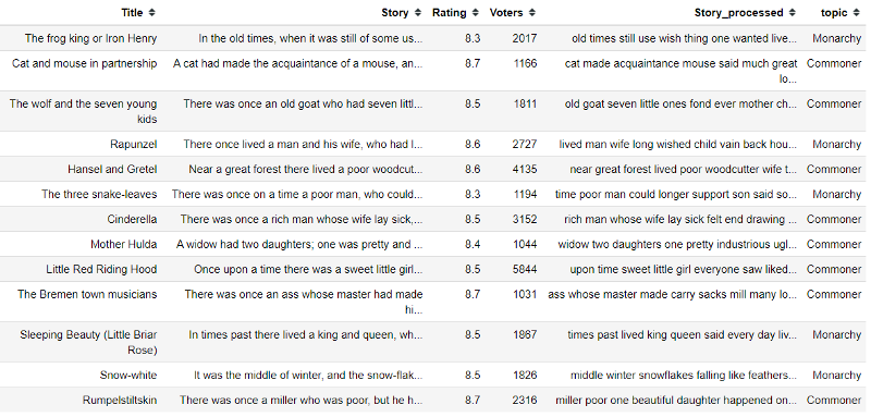
lda_output = best_lda_model .transform(count_data)

df['topic'] = np.argmax(pd.DataFrame(np.round(lda_output,2)).values, axis=1)

df['topic'] = df['topic'].apply(lambda x: 'Monarchy' if x == 0 else 'Commoner')

df.head()

We can see some of the Tales examples that were Monarchy topic or Commoner topic. We can try to take a bigger sample to see what kind of Tales are included in each topic.

df[df['topic'] == 'Monarchy']['Title'].sample(20)

Some of the famous Tales are in the Monarch topic, such as Snow-white and Rapunzel. Let’s see how about the Commoner topic.

df[df['topic'] == 'Commoner']['Title'].sample(20)

In the Commoner topic, we obviously have one of the most famous Tales, Cinderella.

Interestingly, each topic is represented with the famous Tales, but let’s see its general perspective. First, let’s try to visualize the rating and voter distribution.

sns.pairplot(data = df, hue = 'topic')

It seems that the Monarchy topic has a slightly higher rating compared to the Commoner topic. However, the Commoner topic seems to have more voters and thus have more viewers compared to the Monarchy topic.

Let’s us see the basic statistic as well.

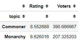
df.groupby('topic').mean()

The information we get from the visualization is similar to the statistic, Monarchy had a slightly higher rating, but Commoner, on average, have more voters.

Let’s see what kind of Tales have higher voters (more than 3000).

Hansel and Gretel, Cinderella, and Little Red Riding Hood; obviously the Fairy Tales you would know because we always read it everywhere. It is interesting because these Commoner tales have a high number of voters.

How about Tales that have quite high voters, let’s say, 1000 voters. What kind of topic they had for that.

df[df['Voters']>1000]

Many of it still dominated by the Commoner Tales and some famous Monarchy Fairy Tales such as Snow-white and Sleeping Beauty.

Conclusion

Some Tales are famous, but it is interesting to see why the Tales are famous. To answer that question, I try to do a topic analysis via LDA and find that the Grimm’s Tales topic could be divided into two fractions; Monarchy and Commoner.

Monarchy topics have a slightly higher rating, but Tales with Commoner topics dominate the number of people reading and voting. This means that Tales with Commoner topic are more famous.

Non-Brand Data

Discussion about this post