Have you heard about the Optimization Problem?

If not, this is the introductory article for the problem.

If not, this is the introductory article for the problem.

Photo by engin akyurt on Unsplash

Introduction

As a Data Scientist, there would be a time that we need to create a script or machine learning model to answer our question. Sometimes, there are many ways to solve our problem. Take an example of a classification problem; we might apply a probability-based model, tree-based model, or linear-based model. Initially, after EDA, we would choose the model with the assumption that filled by the data. Now, maybe we take a Random Forest model and want to train the model.

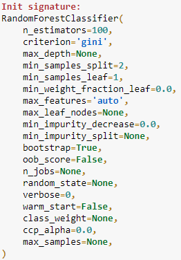
Many of you would realise there are many parameters to tweak, just like in the picture beside. You then try each combination of the parameter until you find the ‘best’ parameter for your model, but it certainly would take a long time.

What I just explained in the passage above is what we called the optimization problem.

Formally, we could define the Optimization Problem as

“The problem of finding the best state according to the objective function.”

What we consider state would be varied as it depends on the context. It could be

• The parameter of the Random Forest Model;

• Chess position on the board;

• Neural network weight in the Deep Learning Model

• Train station placement order on the map.

The important thing here is that there are many possible states, but we want to find the “best” solution (or in the mathematical term objective function, fitness function, cost function, or loss function). For the optimization problem, we want to either maximize or minimize this function.

In the case of the optimization problem, because we compare each state to find the best function mathematically, it means the state should be a numerical value (or numerical vector). Optimization problems itself can be divided into continuous optimization, or discrete optimization depends on the variable.

Mathematical Example

If you have a problem imagining it, let me show it by a simple mathematical function. Imagine if we have an objective function like below.

where x is a vector consisting of the state

Now, for example, we have an optimization problem where we want to maximize the Objective function or, in other words, have the maximum highest value as possible from the function. In our problem above, the function could only take a value between 0 or 1. now, we could have many combinations of x. It could be x = [0,0,0], or x = [0,1,1], etc. but we want to maximize the objective function. It means, the optimal solution would be

where the function with f(x) set to the optimal solution is f(x) = 3. What I just explain is an example of the optimization problem where we want to have an objective function yield the maximum value.

In a real-world problem, the equation would never be that simple. It would often involve a complicated function and an abundant combination of state. It becomes a problem as we cannot optimize the objective function in a reasonable time.

One way to solve this problem is by applying Randomized optimization algorithms. Just like the name implies, we would not go through all the states, but instead, we start at an initial “best” state vector and then randomly generate a new state vector (often a neighbour of the current “best” state). If the new state is better, then the new vector becomes the new “best” state vector. We repeat it until the maximum times or repetition given.

Real Application — Travelling Salesperson Problems

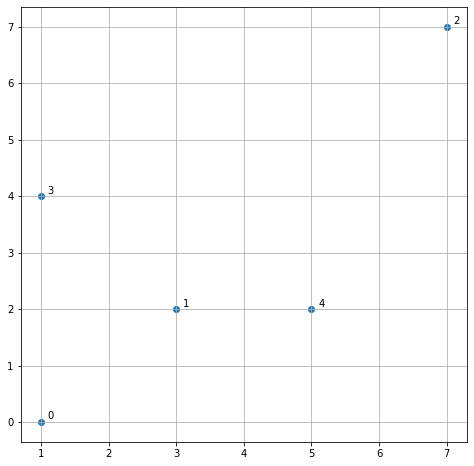
The travelling salesperson problem (TSP) is an optimization problem where we try to determine the shortest tour of the n cities (or house, station, etc. any kind you like), starting and ending at the same point and visiting all of the locations once. For example, I have a collection of five cities in the grid below.

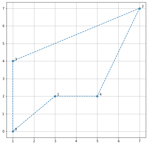
I want the salesperson to travel all the cities exactly once with starting and ending in the same city. If we set the solution vector x = [0,1,2,3,4] and assuming the city start at 0, then the salesman would travel just like in the grid below.

The route travelled seems not the most optimal path. This is where we try to find the shortest route to go or the optimization problem.

For this article, I would use an optimization problem module called mlrose. If you want to install the module, you can run the following code.

#Installing using pippip install mlrose

Solving an optimization problem using mlrose involves three steps:

1. Define a fitness function object (The function we like to minimize/maximize).

2. Define an optimization problem object (Object that contains all of the essential information about the optimization problem we are trying to solve).

3. Run a randomized optimization algorithm.

First, we need to define the fitness function object. Luckily, mlrose already had TravellingSales() class is to be used to define the fitness function object. Initially, TravellingSales() class would need (x, y) coordinates of all the cities (or the distances).

import mlrose

# List of city coordinatescoords = [(1, 0), (3, 2), (7, 7), (1, 4), (5, 2)]

# Initialize fitness function objectfitness_coords = mlrose.TravellingSales(coords = coords)

After initiating the fitness function, we would then define our optimization problem object. The mlrose module already had the TSPOpt() as optimization problem object. We only need to define the object by inputting a few parameters. In the example above, we want to solve a minimization problem of length 5. In that case, we define the optimization object below

# Define optimization problem object. length parameter is the number of the cities, fitness_fn is the fitness function, and we set maximize to false as we want the minimal distance

problem = mlrose.TSPOpt(length = 5, fitness_fn = fitness_coords, maximize=False)

We now ready to select a randomized optimization algorithm and use it to solve our problem. The randomized optimization algorithm is base on the Evolutionary Algorithm, I would not explain the matter in deep, but the parameter used in the mlrose module is based on that. In our example, I try to set the mutation_prob parameter (Just think this parameter as the rate of how big the state to change based on the current best state) to 0.2 and the max_attemps (The repetition number) to 100.

best_state, best_fitness = mlrose.genetic_alg(problem, mutation_prob = 0.2,max_attempts = 100, random_state = 2)

print('Best State is:')print(best_state)

print('Best Fitness (Total Distances) is:')print(best_fitness)

We can see the best state the algorithm found is [1,0,3,2,4]. I also present the Best Fitness to show the total distances we took, as what we minimize in this problem is the total distance (Euclidean Distance to be exact). If we visualize it, our salesman will walk in the following route.

And that’s it. We are already applying the Optimization Problem to our Travelling Salesman Problem and found the best route that the salesman could traverse. This is how we use the Optimization Problem to solve the question we have.

Conclusion

Optimization Problem is the problem of finding the best state according to the objective function. This state could be anything, from the Machine Learning model parameter to the salesman travelling route. The objective is to maximize or minimize our objective function from the given states.