Model Benefit Evaluation with Lift and Gain Analysis

How Lift and Gain analysis could help evaluate the business needs of your model

As Data Scientists, developing machine learning models is a part of our daily job and the reason we are employed in the first place. However, the machine learning models we develop are not merely for show but tools for solving business problems. This is why we need to evaluate our machine learning models — to measure how they impact the business.

Many data scientists measure performance using technical metrics such as Accuracy, Precision, F1 Score, ROC-AUC, etc. These metrics are necessary, but they sometimes do not reflect the model's business-wise effectiveness. Nevertheless, business people need to understand the differences our models would make in business terms compared to random targeting. This is why we use Lift and Gain analysis — to measure how better our prediction model performs than a scenario without the model.

Without further ado, let's get into it.

Lift and Gain Analysis

Lift and Gain analysis evaluates model predictions and their benefits to the business. Although it's often used in marketing target analysis, it's not exclusively so.

The chart below presents the results of a typical Lift and Gain analysis.

Gain and lift charts are visual aids for evaluating the performance of classification models. Unlike the confusion matrix, which evaluates the performance of the entire population, the Gain and Lift chart assesses model performance on a population segment. This means we evaluate the model based on the benefit we could achieve by using it on a portion of the population.

The benefit of Gain and Lift analysis comes from the common business principle that 80% of our revenue often originates from 20% of our customers. This principle is crucial to the decile analysis used in the Gain and Lift chart calculation. The decile analysis is presented in the chart below.

Decile Analysis (Source: http://www.totalcustomeranalytics.com/decile_analysis.htm)

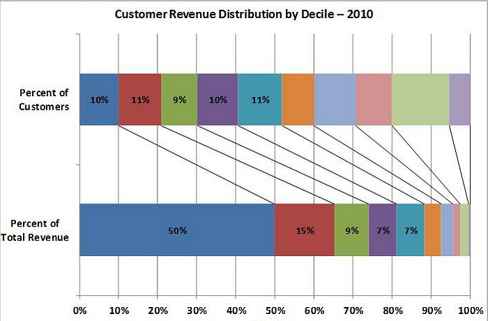
How is Decile Analysis applicable to Gain and Lift analysis? Let's take a few steps back and explain how Gain and Lift analysis is calculated from the beginning.

As previously mentioned, the Gain and Lift chart evaluates the classification model. For the sake of example, let's create a prediction model. In this article, I will use churn data from Kaggle.

import pandas as pd
churn = pd.read_csv('churn.csv')

This dataset has 21 columns, with customer churn being the target variable. This means we will develop a classification prediction model to predict customer churn. For simplicity, I will clean the data for modelling purposes.

# Drop Customer ID
churn = churn.drop("customerID", axis=1)

# Change Ordinal data to numerical
for i in [
    "Partner",
    "Dependents",
    "PhoneService",
    "OnlineSecurity",
    "OnlineBackup",
    "DeviceProtection",
    "TechSupport",
    "StreamingTV",
    "StreamingMovies",
    "PaperlessBilling",
    "Churn",
]:
    churn[i] = churn[i].apply(lambda x: 1 if x == "Yes" else 0)

# OHE categorical data
churn = pd.get_dummies(
    churn,
    columns=["gender", "MultipleLines", "InternetService", "Contract", "PaymentMethod"],
    drop_first=True,
)

# Change object data into numerical
churn["TotalCharges"] = churn["TotalCharges"].apply(
    lambda x: 0 if x == " " else float(x)
)

After cleaning the data, we will attempt to develop the prediction model. For this time, I will use the Logistic Regression model.

# Import the model
from sklearn.model_selection import train_test_split
from sklearn.linear_model import LogisticRegression

# Splitting the model
X_train, X_test, y_train, y_test = train_test_split(
    churn.drop("Churn", axis=1),
    churn["Churn"],
    test_size=0.3,
    stratify=churn["Churn"],
    random_state=101,
)
model = LogisticRegression()
model.fit(X_train, y_train)

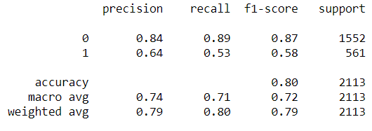
We will conduct our Gain and Lift analysis with our model set to evaluate this model. For comparison, we will also evaluate the model using the usual metrics.

from sklearn.metrics import classification_report
predictions = model.predict(X_test)
print(classification_report(y_test, predictions))

As we can see from the image above, our model's ability to predict churned customers (class 1) is relatively low. Could our model still be beneficial if applied in business? Let's examine this using the Gain and Lift analysis.

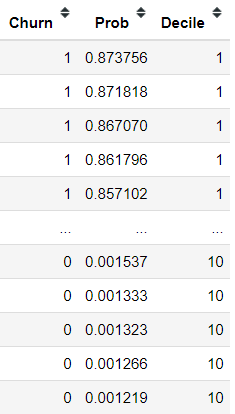
The first step in Gain and Lift analysis is to obtain the model's prediction probability of class 1 based on the test data and sort it in descending order.

#Getting the prediction probability of class 1 and order it by descending order
X_test['Prob']  = model.predict_proba(X_test)[:,1]
X_test = X_test.sort_values(by = 'Prob', ascending = False)
X_test['Churn'] = y_test

Once we have obtained the probabilities and sorted them in descending order, we will divide the data into deciles. This is similar to the decile analysis shown in the image above; we divide the data into ten sets and label them.

# Divide the data into decile
X_test["Decile"] = pd.qcut(X_test["Prob"], 10, labels=[i for i in range(10, 0, -1)])

After dividing the data into deciles, we need to calculate each decile's actual churn (actual class 1, not predicted). I refer to this process as calculating the "Number of Responses."

# Calculate the actual churn in each decile
res = (
    pd.crosstab(X_test["Decile"], X_test["Churn"])[1]
    .reset_index()
    .rename(columns={1: "Number of Responses"})
)
lg = (
    X_test["Decile"]
    .value_counts(sort=False)
    .reset_index()
    .rename(columns={"Decile": "Number of Cases", "index": "Decile"})
)
lg = (
    pd.merge(lg, res, on="Decile")
    .sort_values(by="Decile", ascending=False)
    .reset_index(drop=True)
)

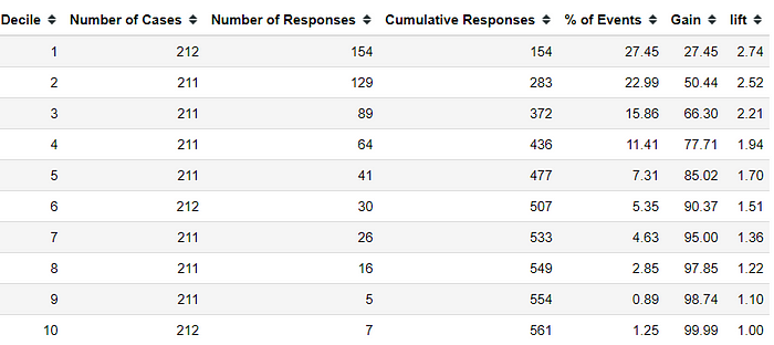
In the image above, we obtain the Number of Cases (the number of data points in each decile) and the Number of Responses (the number of actual positive data points in each decile). With these numbers, we can calculate the Gain value.

Gain is the cumulative Number of Responses (Actual Positives) ratio up to each decile, divided by the total number of positive observations in the data. Let's try to calculate it using our data.

# Calculate the cumulative
lg["Cumulative Responses"] = lg["Number of Responses"].cumsum()

# Calculate the percentage of positive in each decile compared to the total nu
lg["% of Events"] = np.round(
    ((lg["Number of Responses"] / lg["Number of Responses"].sum()) * 100), 2
)
# Calculate the Gain in each decile
lg["Gain"] = lg["% of Events"].cumsum()

From the Gain image above, we can see that the Gain value increases for each decile, but the cumulative total decreases with the higher deciles. So, what is the interpretation of Gain? Gain is the percentage of targets (actual positives) covered at a given decile level.

For example, in the second decile, we had a Gain of 50.44. This means that 50.44% of targets are covered in the top 20% of data, according to the model. In the churn model, we can interpret this as identifying and targeting 50% of customers likely to churn by focusing on 20% of the total customers. From a business perspective, this means that with fewer resources, we could potentially avoid 50% of churn events.

Next, we need to calculate the Lift. The Lift measures how much better we can expect to do with the predictive model compared to a scenario without the model.

lg['Decile'] = lg['Decile'].astype('int')
lg['lift'] = np.round((lg['Gain']/(lg['Decile']*10)),2)

The Lift can be interpreted as the ratio of the gain percentage to the random percentage at a given decile level. In layman's terms, in the second decile, where we have a Lift of 2.52, it means that when selecting 20% of the data based on the model, we could find the target (actual positive) 2.52 times more often than if we randomly selected 20% of the data without using a model.

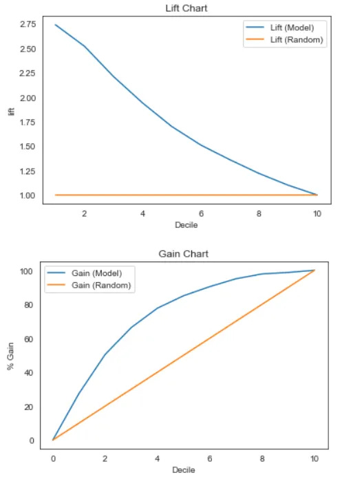
Let's visualize the Gain and Lift chart compared to random selection.

In the image above, we evaluate the model by measuring the Gain and Lift values compared to random selection. The larger the area, the better the model. As the chart shows, our model demonstrates good predictive capabilities because it provides a greater Gain and Lift than random selection. From a business perspective, identifying churn is more effective when using the model, which implies less resource expenditure.

Conclusion

Evaluating models is crucial in data science; however, we must assess the models based on their business utility. It's insufficient to rely solely on technical metrics; we must also consider how our models impact the business. In this article, I have explained how Lift and Gain analysis can be useful in evaluating a model in business terms by using the following:

• Gain value (percentage of target covered in each decile)

• Lift value (ratio of gain percentage to the random percentage at a given decile level)

I hope you find this information helpful!

---

Thank you for reading the Non-Brand Data Newsletter. If you found this helpful post, please share it with your friends. Also, I encourage you to comment on any topics you'd like me to write about!