


Module 1 of the SQL and analytics course. I’ll add the next modules as they are ready.
SQL is often used to answer business questions. However, a request such as “How are sales doing?” still leaves a few things open. We need to decide whether “sales” refers to orders, delivered orders, or revenue before we can write the query.
In my experience, the SQL itself is often not the problem. A query can run correctly and still give us the wrong business number because the population, metric, or time window was never defined.
In this module, we will learn how to turn a general request into a question we can answer with a calculation. We will use monthly sales and repeat purchase rate as examples, then see how the results change as the definition changes.
After this module, you should be able to:
Write a business question with a clear population, metric, and time window
Choose the identifier that matches what you want to count
Check whether every row had enough time to produce the outcome you want to measure
Before we start
Let’s use DB Fiddle for the examples. The tables and every query in this module are already there, so you don’t need an account or a database setup. Run each query as you read, and compare the results with the explanations below them.
The examples use fifteen invented orders based on the Olist customer and order structure. The IDs, statuses, and timestamps were made for this lesson, so they are not direct Olist records. I keep the table small so we can check every row ourselves.
You can also keep the Module 1 SQL script.
Scenario 1: Monthly delivered orders
Let’s start with a common question: How are sales doing? It sounds simple, but we still need to decide what sales means and which period we want to look at.
Start with the order count
Let’s try the first query most people would write. We count every row in the orders table.
SELECT COUNT(*) FROM orders;Before you scroll, try to predict the result. The query runs without errors, but can a single all-time number tell us whether sales are going up or down?

As we can see from the result, the table has fifteen orders. The query is correct, but we still don’t know how sales are doing.
What is still missing
There are three things we still need to decide:
Which orders should we count? The table has orders delivered, cancelled, shipped, and invoiced. We need to decide which of them should count as sales.
What should sales measure? We could count orders, add revenue, or count items sold. These numbers can move differently.
Which period should we use? One all-time total can’t show whether the latest month is higher or lower than the previous month.
This happens because the request doesn’t define the population, metric, or time window. If we make those choices ourselves, another analyst can make different choices and return a different number. Both queries might still be valid.
Define the question
Before we write more SQL, let’s write the question and metric first:
Question: How has the number of delivered orders changed month-by-month across 2017 and 2018?
Metric: Count one order when its status is delivered, then group the count by the month in which the order was placed.
For me, delivered orders are a good starting point because we want completed sales rather than every order attempt. I would calculate revenue separately because refunds and payment timing need their own rules.
Calculate monthly delivered orders
We can use the following query:
SELECT
 date_trunc(’month’, order_purchase_timestamp) AS order_month,
 COUNT(*) AS delivered_orders
FROM orders
WHERE order_status = ‘delivered’
 AND order_purchase_timestamp >= ‘2017-01-01’
 AND order_purchase_timestamp < ‘2019-01-01’
GROUP BY 1
ORDER BY 1;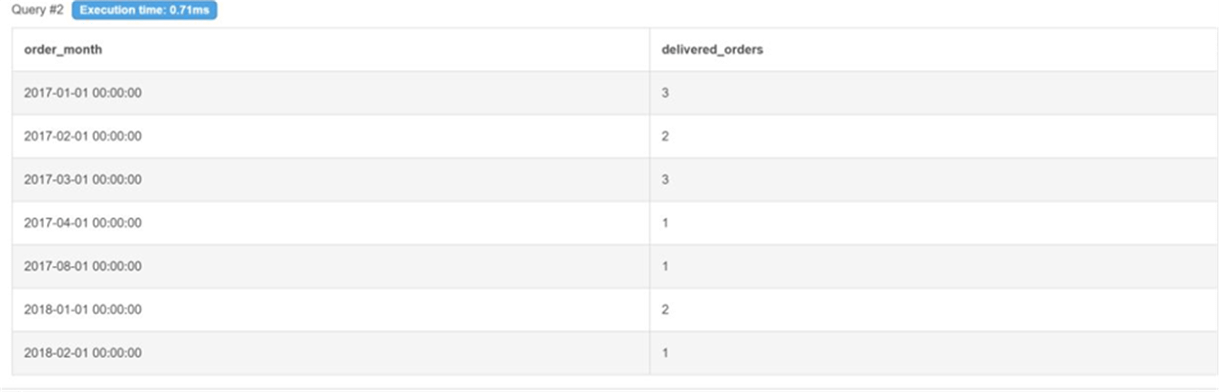
As we can see from the result, we now have a delivered-order count for each month available in the teaching data. Instead of a single total, we have seven rows to compare.
date_trunc(’month’, ...) changes each timestamp to the first day of its month. For example, both 2017-03-02 and 2017-03-22 are treated as 2017-03-01, so they are counted in the same group. GROUP BY 1 refers to the first selected column, so we don’t need to repeat the full expression.
We also use a half-open date range. It includes timestamps on or after 1 January 2017 and stops before 1 January 2019. If we use <= ‘2018-12-31’ instead, an order placed later on 31 December could be left out because the column also contains a time.
There are only seven months in the result because the teaching data doesn’t cover the full two years. We need to check the available dates before we describe the trend.
What changed
We count delivered orders instead of every order status.
We calculate a value per month rather than an all-time total.
The question and the query now use the same definition.
Your call. Delivered orders are not always the right sales metric. You can use all orders or revenue if that matches the question better. The important thing is to write the choice down before calculating the result.
When to break the rule. During early exploration, you might not know the final question yet. That’s fine. Just make it clear that you are exploring and not presenting the result as the final answer.
What to say. “Before I run this, should sales mean orders or revenue, should I include only delivered orders, and which period do you want to compare?”
At this point, you should be able to:
Explain why an order count doesn’t answer every sales question
Define the population, metric, and time window
Compare the written definition with the query
Scenario 2: Repeat purchase rate
Next, let’s look at repeat purchase rate. The metric already has a name, but that doesn’t mean the definition is complete. We still need to decide what counts as a single customer and how long we give someone before they need to order again.
Start with Customer ID
Let’s begin by counting orders for each customer_id.
SELECT
 ROUND(100.0 * COUNT(*) FILTER (WHERE order_count > 1) / COUNT(*), 1) AS repeat_rate_pct
FROM (
 SELECT customer_id, COUNT(*) AS order_count
 FROM orders
 GROUP BY customer_id
) c;
Before you scroll, try to predict the result. What would you think if the repeat purchase rate came back as exactly zero?

As we can see from the result, the repeat rate is 0.0%. This doesn’t mean nobody ordered twice. It means customer_id is not the right identifier for this metric.
Check the customer identifier
In the Olist data model, each order gets a new customer_id. The teaching data follows the same structure, so 15 orders also yield 15 distinct customer_id values.
Because each customer_id appears once, this query can never find a repeat customer. To track the same person across multiple orders, we need the customer_unique_id.
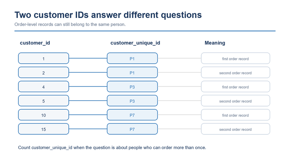
The diagram shows the difference between the two columns. The customer_id identifies the customer record for a single order, while customer_unique_id links multiple order records to the same person in the teaching data.
However, the customer identifier is not the only factor in our decision. We also need to choose the repeat window and decide whether an order must be delivered before it counts as a repeat purchase.
Define the repeat purchase rate
Let’s use this definition:
Metric: Among customers who placed a delivered order, calculate the percentage whose next delivered order was placed within 90 days. Count one customer per customer_unique_id.
Now we have the customer key, order status, and time window. We can use those choices to decide which SQL functions we need.
Calculate the first repeat rate
The following query uses CTEs and window functions. We will cover this in Modules 10 and 11, so you don’t need to write it from scratch yet. For now, look at how each part of the query matches the metric definition.
WITH delivered_orders AS (
 SELECT
 c.customer_unique_id,
 o.order_purchase_timestamp
 FROM orders o
 JOIN customers c ON c.customer_id = o.customer_id
 WHERE o.order_status = ‘delivered’
),
sequenced AS (
 SELECT
 customer_unique_id,
 order_purchase_timestamp,
 ROW_NUMBER() OVER (
 PARTITION BY customer_unique_id
 ORDER BY order_purchase_timestamp
 ) AS order_seq,
 LEAD(order_purchase_timestamp) OVER (
 PARTITION BY customer_unique_id
 ORDER BY order_purchase_timestamp
 ) AS next_order_ts
 FROM delivered_orders
)
SELECT
 ROUND(
 100.0 * COUNT(*) FILTER (
 WHERE next_order_ts IS NOT NULL
 AND next_order_ts <= order_purchase_timestamp + INTERVAL ‘90 days’
 ) / COUNT(*)
 , 1) AS repeat_rate_pct
FROM sequenced
WHERE order_seq = 1;
The first CTE keeps only delivered orders and joins them to customer_unique_id. The second CTE puts each customer’s orders in time order. Then LEAD() finds the next delivered order for the same customer.
Before you scroll, what do you expect now? Should the repeat rate stay at zero or increase?

Compared with the previous result, the rate increases from 0.0% to 20.0%. We fixed the customer identifier, but there is still one problem with the denominator.
Check the 90-day window
To measure a 90-day repeat rate, every customer in the denominator needs 90 days to place another order. A customer who first ordered near the end of the data doesn’t have the same chance as someone who ordered months earlier.
Let’s check how many days each customer had after the first delivered order:
SELECT
 customer_unique_id,
 order_purchase_timestamp AS first_order,
 DATE_PART(’day’, (SELECT MAX(order_purchase_timestamp) FROM orders)
 - order_purchase_timestamp) AS days_they_had
FROM sequenced
WHERE order_seq = 1
ORDER BY days_they_had;
As we can see from the result, one customer first ordered on the final day in the data. Two more customers had only 35 or 40 days. The current denominator counts all three as customers who didn't return, even though we can't observe a full 90-day outcome for them.
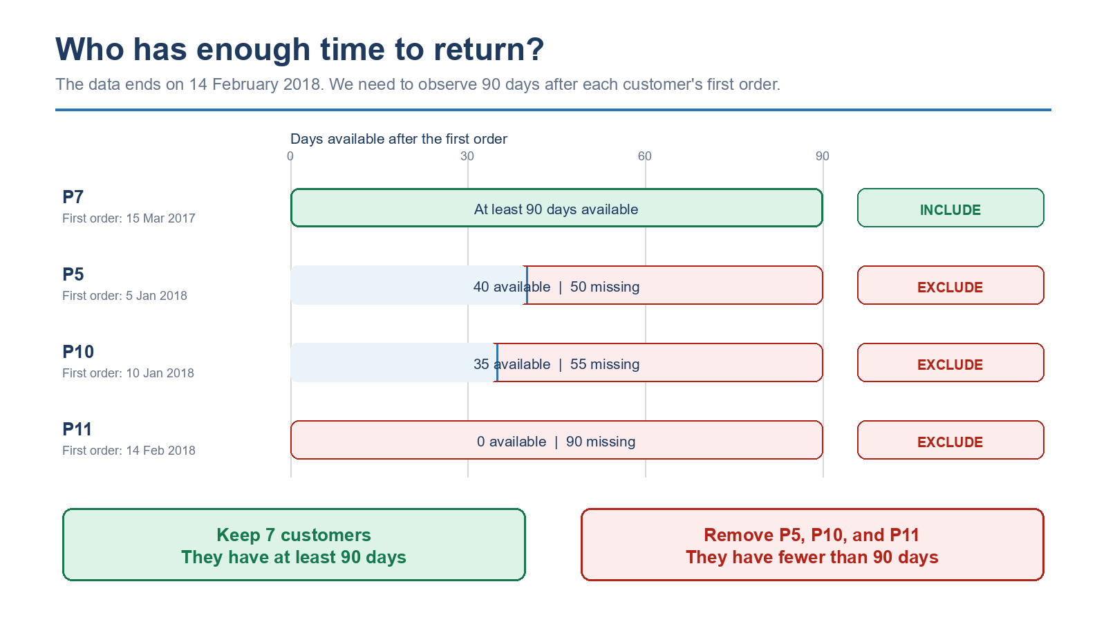
The diagram compares the 90-day window to the end of the data period. Seven customers have a complete observation window, while three need to be removed from the denominator.
Calculate the corrected rate
We can fix the denominator by keeping only customers whose first delivered order was at least 90 days before the final timestamp:
WITH delivered_orders AS (
 SELECT
 c.customer_unique_id,
 o.order_purchase_timestamp
 FROM orders o
 JOIN customers c ON c.customer_id = o.customer_id
 WHERE o.order_status = ‘delivered’
),
sequenced AS (
 SELECT
 customer_unique_id,
 order_purchase_timestamp,
 ROW_NUMBER() OVER (
 PARTITION BY customer_unique_id
 ORDER BY order_purchase_timestamp
 ) AS order_seq,
 LEAD(order_purchase_timestamp) OVER (
 PARTITION BY customer_unique_id
 ORDER BY order_purchase_timestamp
 ) AS next_order_ts
 FROM delivered_orders
)
SELECT
 ROUND(
 100.0 * COUNT(*) FILTER (
 WHERE next_order_ts IS NOT NULL
 AND next_order_ts <= order_purchase_timestamp + INTERVAL ‘90 days’
 ) / COUNT(*)
 , 1) AS repeat_rate_pct,
 COUNT(*) AS customers_counted
FROM sequenced
WHERE order_seq = 1
 AND order_purchase_timestamp + INTERVAL ‘90 days’
 <= (SELECT MAX(order_purchase_timestamp) FROM orders);
The result changes from 20.0% to 28.6%. The first query counted 10 customers, while the corrected one counts 7 customers who had a full 90-day window.
Now we can write the final definition:
Metric: Among customers whose first delivered order was placed at least 90 days before the data ends, calculate the percentage who placed another delivered order within 90 days. Count one customer by customer_unique_id.
What changed
We changed the customer key from
customer_idtocustomer_unique_id.We count only delivered orders before checking for a repeat purchase.
We remove customers who don’t have the full 90 days.
Your call. You still need to decide what one customer means, how long the repeat window should be, and what to do with customers who don’t have the full window. It depends on how the business defines repeat purchasing.
When to break the rule. If only a few customers have incomplete windows and the rate barely changes, you might keep them and state the limitation. Check the difference first.
What to say. “I counted customers by customer_unique_id, included delivered orders, and removed customers who didn’t have a full 90 days to return.”
In an interview. If someone asks how you would measure repeat purchase rate, I wouldn’t start with the window function. I would first define one customer, the qualifying order status, the repeat window, and the observation period. Then I would explain how the query uses each choice.
At this point, you should be able to:
Choose the customer identifier that matches the metric
Make the numerator and denominator follow the same definition
Check whether the available data covers the full measurement window
Manager’s view
When I review an analysis, I would ask for the written question and metric first. That makes it easier to compare the query with what the analyst actually meant to calculate.
For a rate, I would also check the customer key and the time window. If recent customers are counted as failures before they have a chance to return, the rate will be lower than it should be under that definition.
Try it
On the teaching data. Take the request “Which customers are doing well?” and turn it into a question with a population, metric, and time window. Then write what needs to be true about the customers in the denominator.
On your own data. Choose a real request from your work or a dataset you care about. Write the question and metric in the same format, then write one assumption you need to check before calculating it.
Keep the second exercise. It becomes the first page of the analysis you will build through this course.
Keep this
Use the Question and Metric Brief to write down the question, population, metric, time window, decision, and fairness check before opening the SQL editor.
Download the PDF below:

Mark this module complete
Complete one Try-it exercise and save the Question and Metric Brief. Keep it with the SQL and report you build through the rest of the course.
This module counts toward the Certificate of Completion once you complete all 14 modules and their activities. The separate Verified credential requires a finished project and a review against the published rubric.
Next
Module 2: SELECT and FROM: reading the table looks at what one row represents before we count it.
Subscribe to receive the next module when it is published.