The Three Equations Running Every AI You’ve Ever Used
A five-minute tour of the math that powers the popular model you knew.
We live in an era where AI products have become essential tools in various systems and businesses. I am sure you have heard of products like ChatGPT and Google Gemini, or AI functions such as Netflix's recommendation system and the AI companion in Zoom. These tools assist by using the model they're trained on.
As amazing as these products are, their capabilities are derived from foundational mathematical principles. From simple equations to excellent products that change the world
So, what are these equations? Let’s get into it.
Book Recommendation
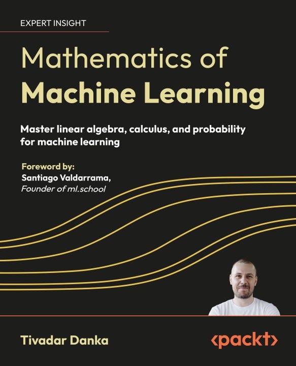
This article was inspired by the Mathematics of Machine Learning book by Tivadar Danka.
This book is the math-first roadmap you wish you had. It explains why math matters in ML and, more importantly, how to apply it in practice.
👉 Curious? You can find the book on this Landing Page
👉Or you can preorder from Amazon.com.
The Dot Product
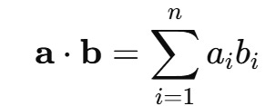
The dot product (or inner product) measures “alignment” between two vectors. At its core, the dot product is a way to combine two vectors into a single number. Formally, the equation is as follows:
It multiplies corresponding elements and sums the results. However, in machine learning, it does something deeper: it measures how much one vector "points in the direction" of another.
In nearly every ML model, from a linear regressor to a transformer, the dot product appears in the same key role:
Where:
x is the input vector (features, image pixels, word embedding)
w is a weight vector learned by the model
b is a bias term (a scalar)
This singular operation serves as the foundation for pattern detection in models. Each weight acts as a filter, enhancing specific input features while diminishing others. Subsequently, the outcome, z, is input into an activation function or softmax to steer the final decision.
Mathematically, when two vectors align, the dot product is large. When they're orthogonal, the dot product is zero. That’s why a high dot product in machine learning can mean "this input matches the pattern the model is looking for."
In Python, it’s easy to perform the dot product. You only need to use the following code:
import numpy as np
np.dot([0.5, 0.2], [0.4, 0.8])
This simple notation is the heart of the model that quietly works to find meaning in your data.
The Gradient
The gradient is the mathematical engine behind learning in machine learning. It tells your model how to adjust its parameters to get better predictions.
Formally, the gradient of a loss function is present as follows:
This vector indicates the direction of the steepest increase in loss. Therefore, to minimize the loss, we move in the opposite direction. This is the fundamental concept behind gradient descent.
Every machine learning model trains by minimizing a loss function, which is a formula that measures the accuracy of its predictions. But how does the model know how to improve? It uses the gradient of the loss with respect to its weights.
In each training step, the model updates its weights as follows:
Where:
θ is the vector of weights
η is the learning rate
∇θL is the gradient vector
This update nudges the weights in the direction that makes the loss go down the fastest.
You rarely calculate the gradient by hand, as libraries like PyTorch already embed gradients within the code.
import torch

x = torch.tensor(2.0, requires_grad=True)
y = x**2 + 3*x
y.backward()
print(x.grad)
The gradient provides machine learning with its feedback loop. It allows the model to “feel” its way toward better performance. Without gradients, we have no means of improving after a wrong prediction.
Bayes’ Rule (and Softmax)
After a model makes a prediction, how do we turn it into a probability we can act on?
There are two core mathematical theories we use for that:
Bayes’ Theorem: the foundation of probabilistic reasoning.
Softmax Function: the standard way neural networks convert scores into probabilities.
They represent the final step in many models, transforming model predictions into confidence values that inform real-world decisions, such as whether to approve a loan, detect a spam email, or translate a word.
Bayes' Rule is a fundamental principle of probability that explains how to adjust your belief in a hypothesis H after observing new data D. Formally, the equation is as follows:
P(H∣D)is the posterior (updated belief after seeing data)
P(D∣H) is the likelihood (how likely the data is under the hypothesis)
P(H)is the prior (belief before seeing the data)
P(D) is the evidence (probability of observing the data under all hypotheses)
In classification tasks, we often want our model to express how confident it is about a prediction. Bayes’ Rule allows us to combine prior knowledge and observed evidence to make more informed decisions.
However, in deep learning, we rarely compute Bayes’ Rule directly. Instead, we often use a function that serves a similar purpose: the softmax function.
Softmax is used in the final layer of neural networks for multi-class classification. It takes a vector of raw scores (called logits) and transforms them into probabilities that sum to 1:
This guarantees that every output value falls between 0 and 1, and that the collective output values create a valid probability distribution.
The differences are that while Bayes’ Rule combines prior probabilities and observed data to produce a posterior, softmax merely normalizes scores into probabilities.
But both aim to answer the same question:
Given what we know, what’s the most likely class?
In Python, we can put perform the Simple Softmax with the following code:
import numpy as np

logits = np.array([2.0, 1.0, 0.1])
exps = np.exp(logits)
probs = exps / np.sum(exps)

print(probs)
Whether you use Bayes’ Rule or softmax, the goal remains to make sense of uncertainty. These mathematical equations allow models to express not only what they predict but also how confident they are, which is a crucial aspect of responsible AI systems.
Conclusion
Behind every AI system lies simple but powerful math. In this article, we have discussed three different equations, including:
The dot product helps models recognize patterns
Gradients help them learn.
Softmax or Bayes’ Rule lets them express confidence.
These equations may be small, but they are fundamental to how machines understand the world. Understanding them would undoubtedly enhance your data work even more.
I hope this has helped!
Mentorship
If you're at a pivotal point in your career or sitting on skills you're unsure how to use, I offer 1:1 mentorship.
It's personal, flexible, and built around you.
For long-term mentorship, visit me here (you can even enjoy a 7-day free trial).


