

A Data Science portfolio is a collection of projects that we use to show our ability to work with data. We can share the work through a GitHub repository or create a website where someone can explore the projects we have developed.
Building the portfolio has become easier with AI as we can use it to help with the code and develop a project from our ideas. This is useful when we are learning a new method because we can spend more time exploring how it works without getting stuck on every part of the implementation.
However, the convenience also brings a question. If AI can help us build the project, what should we show in our Data Science portfolio?
For me, a good portfolio should explain how we approach the problem so someone can understand why we arrived at a particular result. Having a model with high accuracy would not provide much information if we cannot explain what the model predicts or whether the evaluation makes sense.
We don’t need to avoid AI to achieve this. We need to understand the work we present and be able to explain the decisions that affect the result.
In this article, we will explore five public examples to understand what we can include in our own portfolio. Some examples are portfolio websites, while others are individual projects that show how we can explain the work in more detail. We will use them as references without assuming how their authors used AI.
Let’s get into it.
1. Ken Jee’s Data Science Salary Estimator
Let’s start with Ken Jee’s GitHub portfolio, which introduces his projects and links to the repositories where we can explore the implementation. One of the projects is a Data Science salary estimator that uses information from job postings to estimate a salary.
The repository explains how information from job descriptions is prepared for modelling. For example, the project creates features indicating whether certain skills are mentioned in the description. This gives us something to examine because we can follow how the original text becomes information that the model can use.
The project compares the models using Mean Absolute Error or MAE, which measures the average size of the prediction error in the same units as the target. Let’s look at two results reported in the repository.
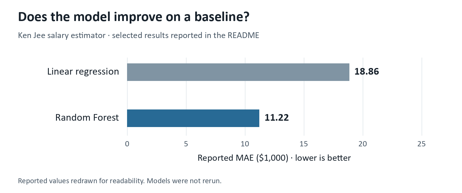
The repository reports an MAE of roughly $18,860 for Linear Regression and $11,220 for Random Forest. This is approximately a 40% reduction in average error relative to the baseline. Showing this comparison gives us a way to discuss whether the more complex model provides an improvement.
We would still need to examine how the evaluation was performed before accepting the result. A lower average error also does not mean that every prediction is within $11,220 of the recorded value.
What should we pay attention to if we develop a similar project?
We need to understand what the salary data represents. A salary estimate from a job posting is not necessarily the salary someone eventually receives. Our explanation should make this clear so the reader understands what we are predicting and how much they can conclude from it.
We could also examine whether the error is similar across job locations. If one location has much less data, the overall MAE might not describe how well the model works there. Comparing the errors alongside the number of examples would help us decide where more data is needed.
AI could help us write the feature extraction code for this project. We would still need to check some job descriptions manually to see whether the extracted information has the meaning we intended. Explaining this check would provide more information about our work than only mentioning that we used AI.
2. Julia Silge’s Animal Crossing Review Analysis
The next example is Julia Silge’s analysis of Animal Crossing reviews. This is a project write-up where we can follow the process of using review text to predict whether the review is good or bad.
The article starts by examining the data before developing the model. Let’s look at the distribution of review lengths.
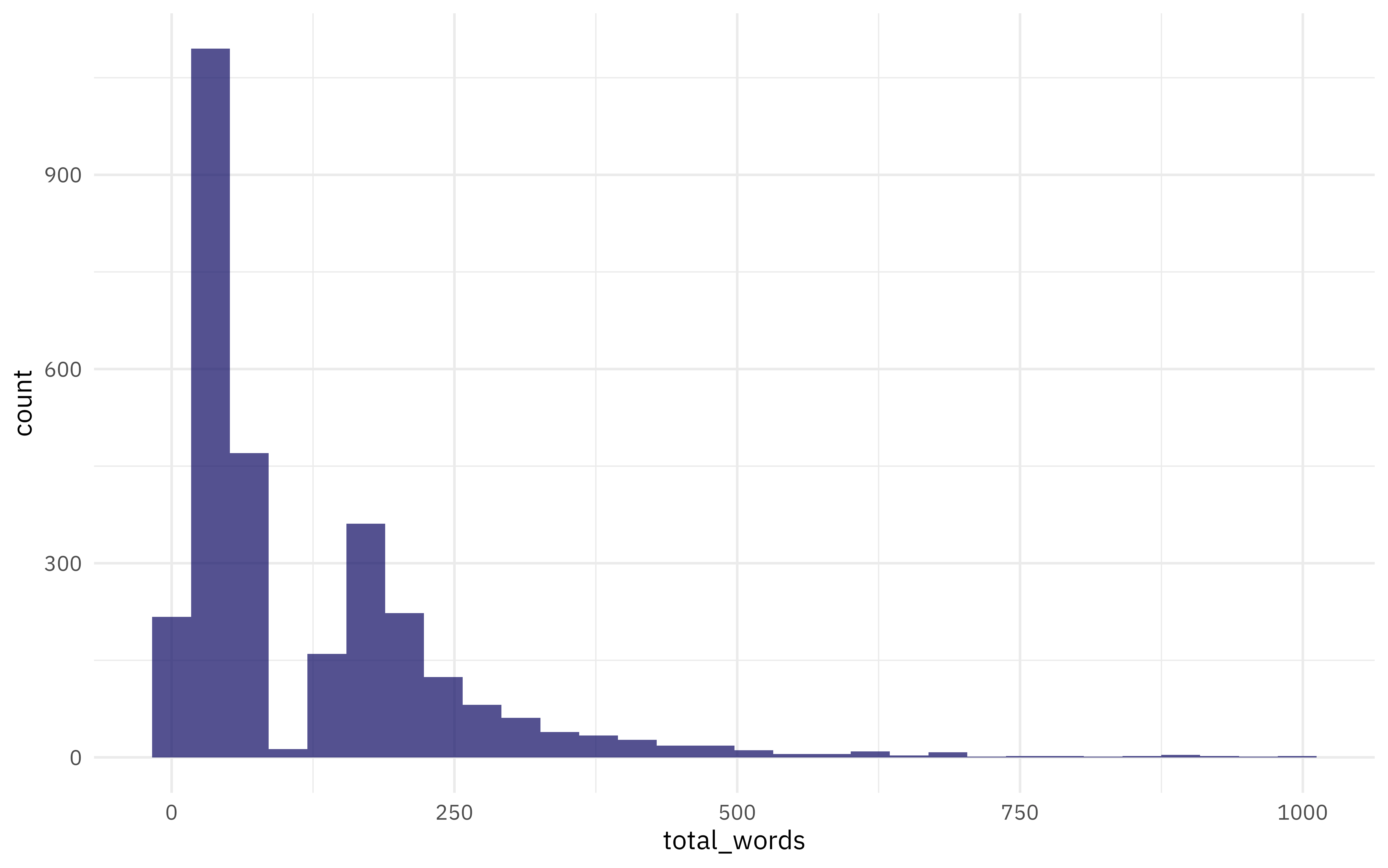
There is a sharp dip around 100 words before the number of reviews rises again. Julia identifies the unusual shape as a possible scraping problem. The chart does not prove what caused it, but it gives us a reason to return to the collection process and check whether some reviews were cut short.
This is something we can include in our own portfolio. We can show the pattern that made us question the data and explain how we checked it before moving on to the model.
The article then compares model settings using several evaluation metrics.
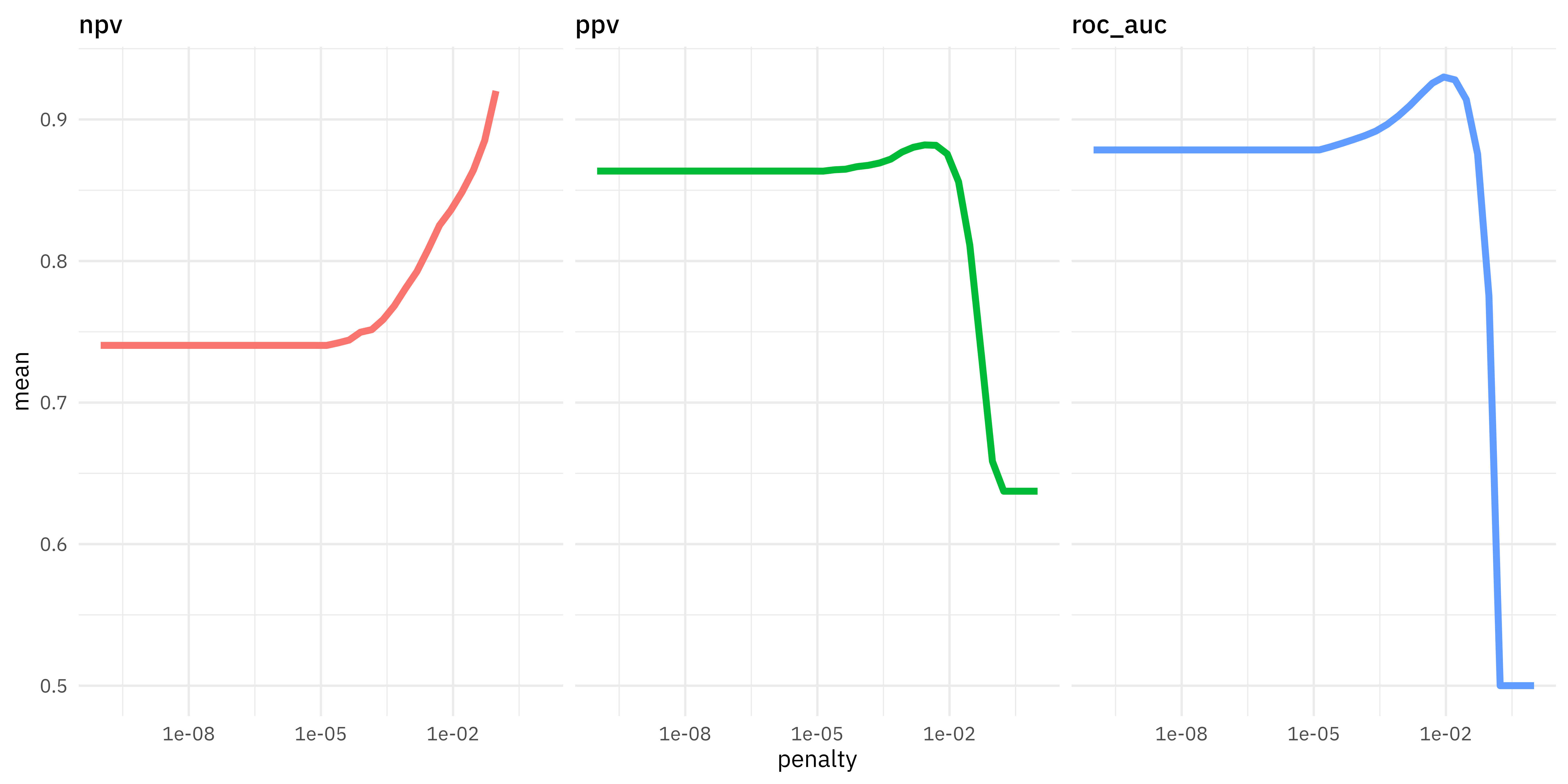
The horizontal axis shows the regularization penalty on a logarithmic scale. Increasing the penalty puts more pressure on the model to shrink its coefficients. We can see that the three metrics respond differently as the penalty becomes larger.
PPV measures how often positive predictions are correct, while NPV does the same for negative predictions. ROC AUC measures how well the model ranks the two classes across thresholds. Near the far right of the chart, NPV increases while PPV and ROC AUC fall sharply. Choosing the largest penalty because one metric improves would therefore miss what happens to the other results. Julia selects the final setting using ROC AUC.
What can we do with an explanation like this?
We can use the same approach when explaining our own classification project. For example, let’s say we want to predict which customers will cancel their subscriptions. We have 1,000 customers in the evaluation data, and 100 of them cancel.
If we predict that every customer stays, the accuracy would be 90% even though we have not identified any customer who cancels. This is why reporting accuracy alone would not explain whether the model is useful for finding cancellations.
Now, suppose the team can only contact 50 customers. We select the 50 customers with the highest predicted risk and find that 20 of them cancel. The precision for this selection would be 40% because 20 out of the 50 selected customers cancel. The recall would be 20% because we found 20 of the 100 cancellations in the evaluation data.
These are example numbers, but they show how we can connect the evaluation to the intended use. We should select the rule using validation data before reporting its performance on untouched test data. You can refer to the Scikit-Learn documentation for more information about the metrics.
We would still need further testing to know whether contacting these customers prevents cancellation. The prediction result only tells us how well we identify the customers who cancel, so our portfolio should explain this limitation as well.
3. Will Koehrsen’s Building Energy Project
Will Koehrsen’s Machine Learning project walkthrough uses building data to predict an Energy Star Score. The work is divided into notebooks that explain the development process and includes a report in the repository.
One part I find useful is the model interpretation notebook, where the author examines a prediction with a large error. Let’s look at the result below.
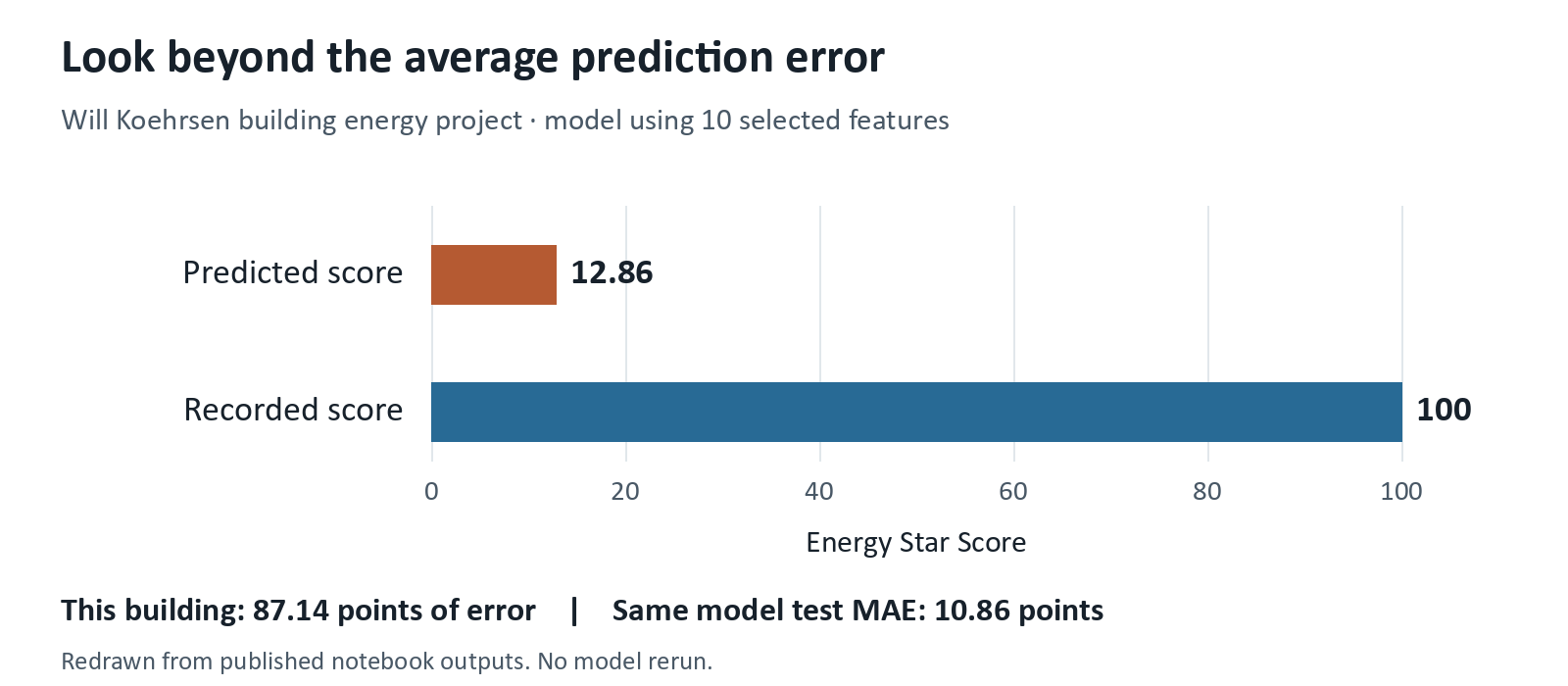
In this example, the model using a reduced set of features predicts approximately 12.86 while the recorded score is 100. The difference is large enough that we would want to investigate what happened instead of only reporting the average error.
The same model has a test MAE of approximately 10.86 points, but the error for this building is 87.14 points. This is why we should examine individual predictions as well as the average.
The notebook then uses LIME to investigate the prediction. LIME approximates the model behaviour around an individual example so we can examine how the inputs contribute to that local explanation.
What can we do with an explanation like this?
We can return to the record and check whether the input was prepared correctly. We could then look for other buildings with similar characteristics to see whether the same error happens repeatedly. This would help us decide whether the problem needs a correction in the data or another modelling experiment.
However, we should remember that explaining a prediction does not prove what causes the real outcome. A feature contributing to a lower predicted score does not automatically mean that changing the feature would change the building’s actual score.
For our own portfolio, we could apply this approach to the largest forecasting errors. If the model often underestimates sales during promotions, we can investigate whether information about promotions was available when making the forecast. We could then test whether including that information improves the validation result.
This gives us a reason for the next experiment based on the errors we observed. If AI helps write the explanation, we should check that it agrees with the actual records before including it in the portfolio.
4. Daniel Bourke’s Amenity Detection Project
Daniel Bourke’s amenity detection project explores using Computer Vision to identify objects in property photos. The project was inspired by Airbnb’s published work and follows the development through to an application.
The final evaluation reports a mean Average Precision, or mAP, of approximately 43.3 across 30 object classes. However, the overall score does not tell us whether the model performs similarly for each type of object. Let’s look at some of the class results.
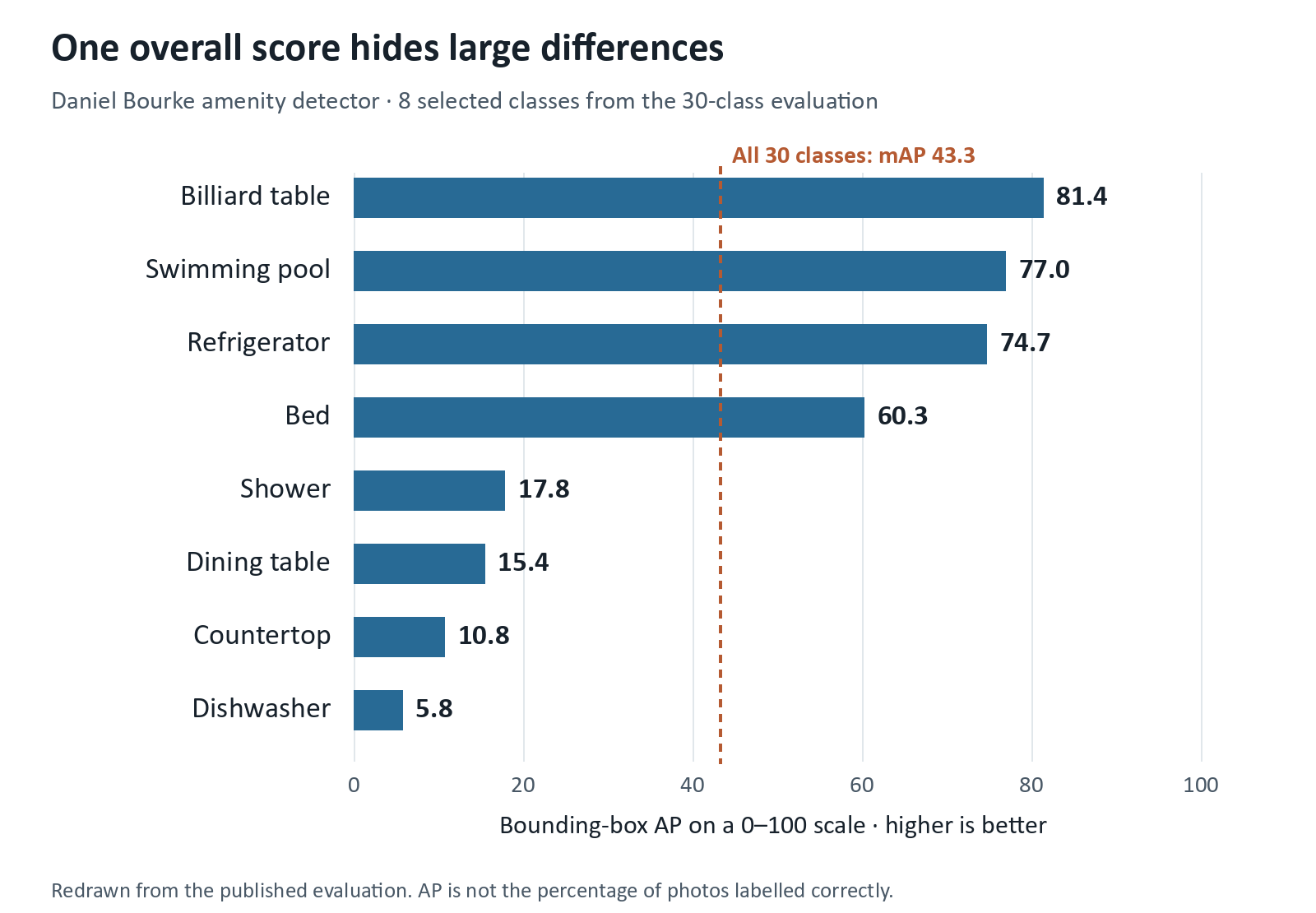
As we can see from the chart, the reported AP is about 74.7 for refrigerators but only 5.8 for dishwashers. These are results from the same evaluation, so the overall mAP would hide a large difference if we reported it alone. AP summarizes detection performance across precision and recall; it is not the percentage of photos where every object is detected correctly.
What would this mean for an application?
If we wanted to use the model to suggest amenities for a property listing, we should investigate the weak categories before relying on the suggestions. We could inspect missed dishwashers and compare them with successful detections to see whether the problem relates to image conditions or the available training examples. We would then test the proposed improvement instead of assuming that adding more data would solve it.
The write-up also reviews the original project goals and acknowledges that the model did not reach the 50 mAP target. It explains that the result cannot be directly compared with Airbnb’s score because the datasets differ. This gives us a useful example of reporting what remains unfinished alongside the application.
We can learn from this when developing an application for our portfolio. A working demonstration shows that we can build the application, but we should also explain the conditions under which we tested it.
For example, we might develop a document classification application that works well with clean PDFs. If someone uploads a scanned page, the application could behave differently because the text needs to be extracted from an image first. Testing both types of documents would give us a better understanding of what the application supports.
We could extend this by checking what happens when the uploaded file is empty or has an unsupported format. The result should help us decide whether the application needs to reject the file or ask someone to review it.
AI can help us develop the interface, but we need these checks to understand whether the workflow behaves as expected. We can explain the remaining limitations in the project documentation and provide instructions for running the application locally if the live version is unavailable.
5. Anthony Lipphardt’s Data Science Portfolio
Our last example is Anthony Lipphardt’s portfolio website. The page introduces his work through project descriptions and provides links for readers who want to explore further.
The collection includes work in exploratory analysis and data visualization as well as Machine Learning. This shows how we can use a portfolio to present different types of work without making every project a prediction model.
How should we select the projects for our own portfolio?
I would start by considering what we want someone to understand about our ability. If several projects repeat the same modelling process on a clean dataset, they might not show how we deal with other parts of a Data Science problem.
For example, we could develop a retail analysis that examines repeat purchases using SQL. The explanation would include how we handled returned orders so the reader can understand how the repeat purchase measure was calculated.
We could then include a demand forecasting project that compares the model with a simple seasonal forecast. This would give us another type of work to discuss because we need to explain whether the model improves on an approach that is already easy to use.
These are suggestions for our own projects rather than examples taken from Anthony’s website. The idea is to select work that adds something different to the collection while keeping the detailed explanation accessible through the project links.
We can use a short introduction on the portfolio page to explain the question each project addresses. Someone interested in the result can then open the notebook or report to understand the work further. This also means we can improve the project explanation without making the portfolio’s main page too long.
Developing the Portfolio with AI
The examples above give us different ways to explain our work. We can apply the same approach when AI is part of the development process or when the project itself uses an AI model.
Let’s say we build an application that answers questions from documents. Showing a successful answer would be a good demonstration, but we would need more examples to understand whether the application works consistently.
We could prepare questions with the passages that should support the answers. We can then check whether the application finds the correct passage before examining whether the answer agrees with it. If the application finds the wrong passage, changing the answer prompt alone might not fix the problem.
Additionally, we should include questions that the documents cannot answer. This would let us examine whether the application acknowledges the missing information or provides an answer without support. We can use the same set of questions when testing a change so the comparison is easier to follow.
For AI-assisted coding, the explanation should focus on how we checked the output. For example, we might use AI to help merge customer data and then discover that the merge creates several rows for the same customer. Comparing the customer counts before and after the merge would help us identify the problem and correct the analysis.
GitHub’s Copilot guidance also recommends reviewing and testing generated code. In a Machine Learning project, we should check that preprocessing does not learn from the test data. The Scikit-Learn data leakage guide explains how this can lead to an overly optimistic evaluation.
If I were reviewing the portfolio, I would use these explanations to discuss why the author chose an approach and what they would investigate next. That is how I would recommend using a portfolio in a discussion, although each company can have a different evaluation process.
We don’t need to replace an existing project every time a new tool becomes available. We can start by revisiting a result that we have not explained well and investigate why it happened. The work we add through that investigation can help someone understand our ability even when AI assists with the implementation.
Continue Learning with Non-Brand Data
If you are interested in learning more about Data Science, Machine Learning, and AI, you can subscribe to Non-Brand Data. I regularly share articles, experiments, and examples that we can learn from.
For readers who want to explore a subject in more detail, the paid subscription also includes in-depth tutorials, written courses, notebooks, code, and additional learning materials.
I also offer 1-on-1 mentorship through MentorCruise if you want to discuss your learning direction, Data Science projects, technical challenges, or career development.